Depressurized Loss of Forced Cooling Transient (DLOFC)

The DLOFC transient simulation was initiated by (Reitsma et al., 2013):

1. Reducing the mass flow rate of the coolant linearly from its nominal value to zero over thirteen seconds.

2. The system pressure was reduced linearly from 7.0 MPa to atmospheric pressure (0.101 MPa).

3. the control rods were fully inserted (SCRAM) to shutdown the reactor after completing the flow rate and pressure ramps.

4. Beyond that, there were no changes to the system's main parameters, and the simulation was performed for up to 140 hours.

During the DLOFC transient simulation, coupled neutronics and thermal-hydraulics calculations were performed and the following progression of the reactor parameters was observed during the transient:

1. The reactor power starts decreasing at the beginning of the transient due to the negative thermal feedback.

2. The prompt power goes to zero while the remaining reactor power is just the decay heat component of the fuel.

3. The maximum fluid and solid temperatures start moving axially and toward the top of the core.

4. Temperature distributions change mainly in the radial direction, and there is a significant change in the solid temperature of the reflector and RPV regions.

5. The maximum fuel temperature reaches 1503.26 °C (1776.41 K) during DLOFC transient compared to the reference results which is around 1500 °C (Zheng et al., 2018) and (Strydom, 2008).

The set of input files to run the DLOFC can be thought of as the left hand side of the app setup show in Figure 1.

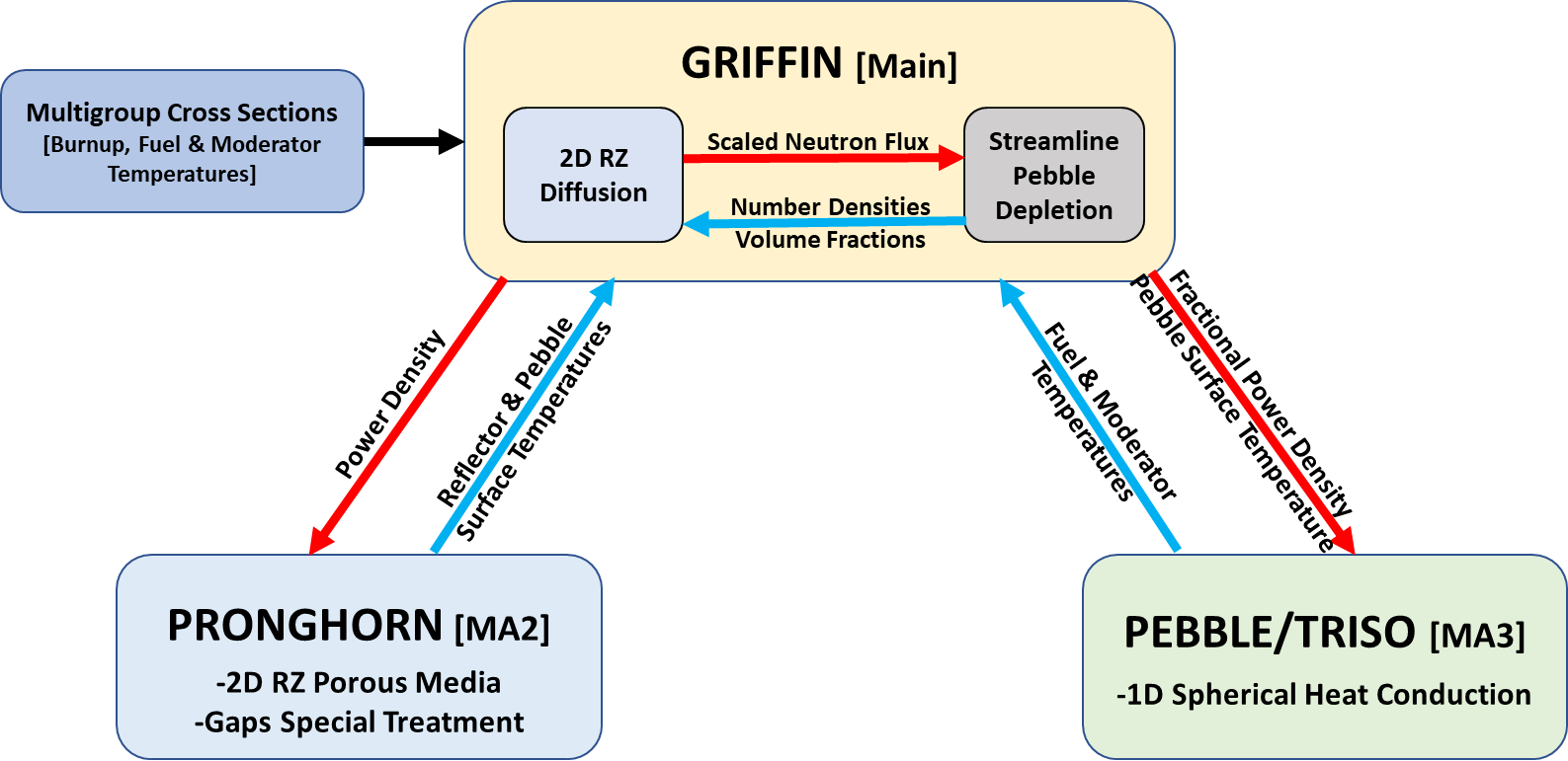
Figure 1: Schematic of the application setup for the DLOFC case.

Thus, two inputs are required for this problem. These are the htr_pm_neutronics_tr_dlofc.i and htr-pm-flow-fv-tr-dlofc.i The first input sets the neutronics calculations and calls the second input which performs the Pronghorn calculations. The neutronics input is mostly similar to the input in the neutronics section model. The major difference is in the MultiApps block in which the pebble/Triso conduction solution is eliminated compared to the steady state input htr_pm_neutronics_ss.i.

[MultiApps]
  [flow]
    type = TransientMultiApp
    input_files = 'htr-pm-flow-fv-tr-dlofc.i'
    positions = '0 0 0'
    execute_on = 'TIMESTEP_END'
  []
[]

For the reader's information, Mesh is imported from a previous run instead of redefining it.

[Mesh]
  [file]
    type = FileMeshGenerator
    # for single-physics simulation restart (as the parent app)
    # file = 'htr-pm-flow-fv-ss_out.e'
    # use_for_exodus_restart = true
    # for multiphysics simulation restart (as a multiapp)
    # We use the checkpoint to make sure to use the same partitioning
    file = 'htr_pm_griffin_ss_out_flow0_cp/LATEST'
  []
  coord_type = RZ
[]

The Physics block, variables are imported from the Exodus file. Notice velocity_variable, pressure_variable, and fluid_temperature_variable definition in Physics.

[Physics]
  [NavierStokes]
    [Flow]
      [all]
        # exodus restart
        # initialize_variables_from_mesh_file = true

        # basic settings
        block = ${fluid_blocks}
        compressibility = 'weakly-compressible'
        gravity = '0.0 -9.81 0.0'

        # Variables, defined below for the Exodus restart
        velocity_variable = 'superficial_vel_x superficial_vel_y'
        pressure_variable = 'pressure'

        # Porous treatement
        porous_medium_treatment = true
        friction_types = 'darcy forchheimer'
        friction_coeffs = 'Darcy_coefficient Forchheimer_coefficient'
        use_friction_correction = true
        consistent_scaling = ${scaling}
        porosity_smoothing_layers = 0

        # fluid properties
        density = 'rho'
        dynamic_viscosity = 'mu'

        # boundary conditions
        inlet_boundaries = 'reactor_inlet'
        momentum_inlet_types = 'flux-mass'
        flux_inlet_pps = 'set_inlet_mfr'
        flux_inlet_directions = '0 1 0'

        outlet_boundaries = 'reactor_outlet'
        momentum_outlet_types = 'fixed-pressure'
        pressure_functors = 'pressure_out_fn'

        wall_boundaries = 'pbed_inner pbed_outer hot_plenum_walls cold_plenum_walls riser_walls bypass_wall'
        momentum_wall_types = 'symmetry   slip       slip             slip              slip        slip'

        # numerical parameters
        pressure_face_interpolation = average
        momentum_advection_interpolation = upwind
        mass_advection_interpolation = upwind
        # prevents solution jump on future restarts
        time_derivative_contributes_to_RC_coefficients = false
      []
    []
    [FluidHeatTransfer]
      [all]
        # exodus restart
        # initialize_variables_from_mesh_file = true

        fluid_temperature_variable = 'T_fluid'
        block = ${fluid_blocks}

        # material properties
        thermal_conductivity = 'kappa'
        specific_heat = 'cp'

        # convective heat transfer
        ambient_convection_blocks = '1 2 3 5 6 61 71'
        ambient_convection_alpha = 'alpha'
        ambient_temperature = 'T_solid'

        # boundary conditions
        # see Flow physics for list of boundaries
        energy_inlet_types = 'flux-mass'
        energy_inlet_functors = '${T_inlet}'

        energy_wall_types = 'heatflux   heatflux   heatflux         heatflux          heatflux    heatflux'
        energy_wall_functors = '0          0          0                0                 0           0'

        # numerical parameters
        energy_advection_interpolation = upwind
        energy_scaling = 5e-6
        coupled_flow_physics = 'all'
        system_names = 'nl0'
      []
    []
  []
[]

Additional initial conditions are imported from previous run as in the Variables block.

[Variables]
  [T_solid]
    type = INSFVEnergyVariable
    block = '${solid_blocks}'
    # restart from exodus
    # initial_from_file_var = T_solid
    # initial_from_file_timestep = LATEST
  []
[]

The most important difference between the steady state and the transient case calculation is the fact that the transient case (i.e. DLOFC) changes the boundary conditions to mimic the DLOFC, while the steady state case is run with eigenvalue for neutronics and in "transient" mode for other physics until the calculation is converged to the steady state solution. The pressure, temperature, mass flow variations are defined in the Functions block as follows

[Functions]
  # viscosity was ramped in equilibrium calculation
  [mu_ramp_fn]
    type = PiecewiseLinear
    x = '0  1 1e+7'
    y = '1  1 1'
  []
  # DLOFC transient
  [mfr_fn]
    type = PiecewiseLinear
    x = '    0    1       13'
    y = ' ${mfr}  ${mfr}  0.0'
  []
  [pressure_out_fn]
    type = PiecewiseLinear
    x = '  0          1           13'
    y = '${p_outlet}  ${p_outlet} 101325.0'
  []
  # increase time steps as transient slows down
  [dt_max_fn]
    type = PiecewiseLinear
    x = '-10 0 16 30 1000 5000 20000 100000 200000 500000'
    y = '  1 1 1  1  50   100  200   400   400   500'
  []
[]

Results

The fluid temperature distribution at different time steps of the transient are in Figure 2. The pebble surface temperature distribution as a function of time is shown in Figure 3.

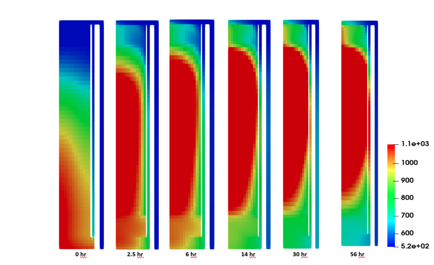
Figure 2: Fluid temperature distribution as a function of time in DLOFC accident condition

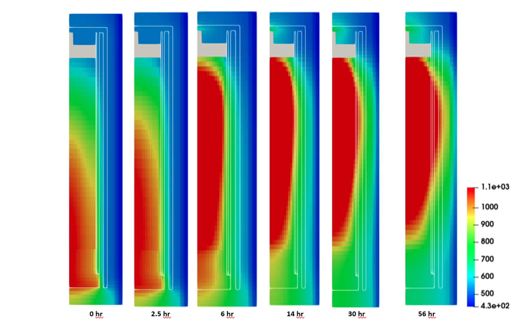
Figure 3: Pebble surface temperature distribution as a function of time in DLOFC accident condition

Input Execution

The execution lines for the equilibrium core calculations, null transient, and DLOFC transient

1. mpirun -np 48 blue_crab-opt -i htr_pm_neutronics_ss.i

2. mpirun -np 48 blue_crab-opt -i htr_pm_neutronics_tr_null.i

3. mpirun -np 48 blue_crab-opt -i htr_pm_neutronics_tr_dlofc.i

Note that the steady state solution should be provided before running any transient calculations to setup initial conditions.