Griffin Open Xe-100 Results

The result files include the binary files from the steady-state case, which serve as initial conditions for the null and IQS cases; the pke_params csv files from the null and IQS cases that contain the generated PKE parameters; the regular csv files which contain regular output from the steady-state, null, and IQS cases; and the pke_fuel_auto csv which is output from the PKE case. This contains the results of the reproduction of the temperature transient in the IQS case.

A brief summary of the results for the SPH-corrected cross sections follows. For a more detailed explanation, see Stewart et al. (Stewart et al., 2022).

Steady-State Results

The steady-state $var element = document.getElementById("moose-equation-5fb7b6be-e007-4b75-9e4b-98626c468074");katex.render("k_{eff}", element, {displayMode:false,throwOnError:false});$ generated by Griffin for the constant temperature of $var element = document.getElementById("moose-equation-3af82124-610c-4462-8b6c-1e8946e0df0d");katex.render("900 K", element, {displayMode:false,throwOnError:false});$ was 1.32988. This was compared to the Serpent model for this same reactor, which had a $var element = document.getElementById("moose-equation-a5794b26-0e46-4cbc-a830-2a0f201064a3");katex.render("k_{eff}", element, {displayMode:false,throwOnError:false});$ of 1.32987 with an uncertainty of 4.3E-05. Therefore, the Griffin-calculated $var element = document.getElementById("moose-equation-83d1e386-7d72-4ae2-83ce-79b26a1a1ecd");katex.render("k_{eff}", element, {displayMode:false,throwOnError:false});$ was within the statistical uncertainty of the Serpent value, once SPH factors were computed and applied.

The steady-state scalar and adjoint fluxes are show in Figure 1.

Fluxes and power density calculated from the constant temperature model (900 K). [!citep](Stewart2022).

Figure 1: Fluxes and power density calculated from the constant temperature model (900 K). (Stewart et al., 2022).

PKE Parameters and Reactivity Coefficients

Generated PKE parameters compared with Serpent values are shown in Table 1.

Table 1: Comparison of PKE parameters at $var element = document.getElementById("moose-equation-32a2c378-30d4-4d30-ae74-ae0c4789fdbd");katex.render("900 K", element, {displayMode:false,throwOnError:false});$ using super-homogenization corrected cross sections (Stewart et al., 2022).

	$var element = document.getElementById("moose-equation-a2a5fc00-fdf5-4ec3-af78-ec4b33f477b7");katex.render("\\beta_1", element, {displayMode:false,throwOnError:false});$	$var element = document.getElementById("moose-equation-38d38de0-c745-41d7-ad4c-eda8ea647d57");katex.render("\\beta_2", element, {displayMode:false,throwOnError:false});$	$var element = document.getElementById("moose-equation-bfe3b3c0-c976-4eb8-9202-ab7b5ef0627c");katex.render("\\beta_3", element, {displayMode:false,throwOnError:false});$	$var element = document.getElementById("moose-equation-a69fe9cb-bb8a-43cc-b221-cd93330a9223");katex.render("\\beta_4", element, {displayMode:false,throwOnError:false});$	$var element = document.getElementById("moose-equation-afa5cacd-f880-41f3-be65-26c0805aacea");katex.render("\\beta_5", element, {displayMode:false,throwOnError:false});$	$var element = document.getElementById("moose-equation-b3cbf1fc-4f1d-4e5b-8783-2262677d5f7e");katex.render("\\beta_6", element, {displayMode:false,throwOnError:false});$
Serpent	$var element = document.getElementById("moose-equation-1a5813b3-8dd0-4b13-949e-2b91046091e9");katex.render("2.319E-4", element, {displayMode:false,throwOnError:false});$	$var element = document.getElementById("moose-equation-9d6b10e0-a6d3-41d9-969a-4dfa5aca9693");katex.render("1.202E-3", element, {displayMode:false,throwOnError:false});$	$var element = document.getElementById("moose-equation-6638e2c3-67b9-4307-88a3-54dee4d0f973");katex.render("1.143E-3", element, {displayMode:false,throwOnError:false});$	$var element = document.getElementById("moose-equation-b90470f2-4f93-47cf-8ee4-fbd0979438fe");katex.render("2.576E-3", element, {displayMode:false,throwOnError:false});$	$var element = document.getElementById("moose-equation-d053d525-7074-422f-9171-8489023b3062");katex.render("1.066E-3", element, {displayMode:false,throwOnError:false});$	$var element = document.getElementById("moose-equation-4bad45de-8b1a-40ca-b312-a31047fd6642");katex.render("4.465E-4", element, {displayMode:false,throwOnError:false});$
Griffin	$var element = document.getElementById("moose-equation-f3d04745-fb83-4d89-811c-a600e3d46692");katex.render("2.344E-4", element, {displayMode:false,throwOnError:false});$	$var element = document.getElementById("moose-equation-e254ca66-691e-4fbd-abc0-ece0149c183e");katex.render("1.210E-3", element, {displayMode:false,throwOnError:false});$	$var element = document.getElementById("moose-equation-a2644db2-7e26-4f71-a6bf-ada7a9f871cd");katex.render("1.150E-3", element, {displayMode:false,throwOnError:false});$	$var element = document.getElementById("moose-equation-7397391a-3120-45d8-8747-1a232c5d8d3a");katex.render("2.588E-3", element, {displayMode:false,throwOnError:false});$	$var element = document.getElementById("moose-equation-1b4ef063-a884-4225-82b6-9768ad983756");katex.render("1.070E-3", element, {displayMode:false,throwOnError:false});$	$var element = document.getElementById("moose-equation-c0a88c85-5975-455e-9f32-5a5939b9b0f1");katex.render("4.486E-4", element, {displayMode:false,throwOnError:false});$
Diff. (%)	$var element = document.getElementById("moose-equation-c0a41bca-be92-4299-b83f-00c371139714");katex.render("-1.052", element, {displayMode:false,throwOnError:false});$	$var element = document.getElementById("moose-equation-21a1a6e0-2dbf-4ec1-b664-cc7c718d808f");katex.render("-0.675", element, {displayMode:false,throwOnError:false});$	$var element = document.getElementById("moose-equation-d9781814-7af7-4ced-8f7c-9496ccd989e9");katex.render("-0.691", element, {displayMode:false,throwOnError:false});$	$var element = document.getElementById("moose-equation-d64221cb-686e-4006-a468-7987460b7769");katex.render("-0.469", element, {displayMode:false,throwOnError:false});$	$var element = document.getElementById("moose-equation-a8923f8b-c2bf-421d-8275-22d5a0685165");katex.render("-0.465", element, {displayMode:false,throwOnError:false});$	$var element = document.getElementById("moose-equation-f720e7f5-645d-440d-b3f5-ef890a30fc56");katex.render("-0.469", element, {displayMode:false,throwOnError:false});$
	$var element = document.getElementById("moose-equation-7f63dcd6-2455-43e5-9825-a021da18a769");katex.render("\\lambda_1", element, {displayMode:false,throwOnError:false});$	$var element = document.getElementById("moose-equation-f0ac894a-8e2a-4d80-8c05-29d7ab0c8f84");katex.render("\\lambda_2", element, {displayMode:false,throwOnError:false});$	$var element = document.getElementById("moose-equation-1983eb2a-ff22-4d6d-8e2a-89833f618ce2");katex.render("\\lambda_3", element, {displayMode:false,throwOnError:false});$	$var element = document.getElementById("moose-equation-5b1adbce-85ac-47e1-81df-ed1d5644a176");katex.render("\\lambda_4", element, {displayMode:false,throwOnError:false});$	$var element = document.getElementById("moose-equation-ce71ea64-031d-4a0a-b220-254f4d0ef203");katex.render("\\lambda_5", element, {displayMode:false,throwOnError:false});$	$var element = document.getElementById("moose-equation-8d9224d4-a4c7-4a38-897e-7e9b013b6d8f");katex.render("\\lambda_6", element, {displayMode:false,throwOnError:false});$
Serpent	$var element = document.getElementById("moose-equation-794c9416-2528-493a-b93f-fde6a5039ff3");katex.render("1.334E-2", element, {displayMode:false,throwOnError:false});$	$var element = document.getElementById("moose-equation-73b48b07-a397-488d-a143-1a602fba6b0e");katex.render("3.273E-2", element, {displayMode:false,throwOnError:false});$	$var element = document.getElementById("moose-equation-109d5abd-29e6-41fc-a243-ce3100ef6d95");katex.render("1.208E-1", element, {displayMode:false,throwOnError:false});$	$var element = document.getElementById("moose-equation-be5cf5f4-a6fe-437e-8583-3c7a3ecfa779");katex.render("3.029E-1", element, {displayMode:false,throwOnError:false});$	$var element = document.getElementById("moose-equation-5bb44ea0-4719-47fb-a52f-5be68a8fd67e");katex.render("8.501E-1", element, {displayMode:false,throwOnError:false});$	$var element = document.getElementById("moose-equation-5ea679eb-4e83-458e-8274-9b961caede25");katex.render("2.855", element, {displayMode:false,throwOnError:false});$
Griffin	$var element = document.getElementById("moose-equation-3efcfada-35d6-46fd-aa97-4adb2e3cfa1a");katex.render("1.334E-2", element, {displayMode:false,throwOnError:false});$	$var element = document.getElementById("moose-equation-4bb6c78e-dad3-4fc8-b681-e6567356a590");katex.render("3.273E-2", element, {displayMode:false,throwOnError:false});$	$var element = document.getElementById("moose-equation-8e5384bf-da0f-4840-8a23-ed88b0f9b95c");katex.render("1.208E-1", element, {displayMode:false,throwOnError:false});$	$var element = document.getElementById("moose-equation-908b0856-6d21-41e9-9f21-6ec2bc0998a7");katex.render("3.029E-1", element, {displayMode:false,throwOnError:false});$	$var element = document.getElementById("moose-equation-32b805c6-517e-4445-8a8d-88fbb59a794a");katex.render("8.501E-1", element, {displayMode:false,throwOnError:false});$	$var element = document.getElementById("moose-equation-1680c0a4-e816-499e-85bb-5a839cfee272");katex.render("2.855", element, {displayMode:false,throwOnError:false});$
Diff. (%)	$var element = document.getElementById("moose-equation-4c88e319-e8eb-4189-968b-a0d0f885dc56");katex.render("< 0.001", element, {displayMode:false,throwOnError:false});$	$var element = document.getElementById("moose-equation-20e69dec-fc6d-4b28-bdec-973ea1330202");katex.render("< 0.001", element, {displayMode:false,throwOnError:false});$	$var element = document.getElementById("moose-equation-11919352-8cde-4e2b-a253-40a7c46e6192");katex.render("< 0.001", element, {displayMode:false,throwOnError:false});$	$var element = document.getElementById("moose-equation-5b3e12a2-f33d-4acf-81cb-b965e67d3c84");katex.render("< 0.001", element, {displayMode:false,throwOnError:false});$	$var element = document.getElementById("moose-equation-0cacb5d2-11aa-4e37-8e36-e72aa411a2c4");katex.render("< 0.001", element, {displayMode:false,throwOnError:false});$	$var element = document.getElementById("moose-equation-4a50e849-3a4f-4514-9117-2df4d9d870da");katex.render("< 0.001", element, {displayMode:false,throwOnError:false});$
	$var element = document.getElementById("moose-equation-d6409683-ccb1-43aa-a93d-e98bceac8995");katex.render("\\beta_{total}", element, {displayMode:false,throwOnError:false});$	$var element = document.getElementById("moose-equation-4a509444-f549-4890-b457-d7e53e8353d9");katex.render("\\lambda_{total}", element, {displayMode:false,throwOnError:false});$	$var element = document.getElementById("moose-equation-d7d050a4-0608-4a43-bd83-b5c7f5427e8e");katex.render("\\Lambda", element, {displayMode:false,throwOnError:false});$
Serpent	$var element = document.getElementById("moose-equation-46994d8b-9cca-4c2e-8941-d58929a6fd65");katex.render("6.434E-3", element, {displayMode:false,throwOnError:false});$	$var element = document.getElementById("moose-equation-b6520771-c8bb-453c-84e9-f57911611dc3");katex.render("4.162", element, {displayMode:false,throwOnError:false});$	$var element = document.getElementById("moose-equation-278e71bd-44fd-4f66-8092-314b70141da6");katex.render("5.116E-4", element, {displayMode:false,throwOnError:false});$
Griffin	$var element = document.getElementById("moose-equation-ed265f15-e596-4953-a1c7-06eeff0034e5");katex.render("6.467E-3", element, {displayMode:false,throwOnError:false});$	$var element = document.getElementById("moose-equation-6e9ba07b-4180-4858-ac00-1bf4c4326fd7");katex.render("4.162", element, {displayMode:false,throwOnError:false});$	$var element = document.getElementById("moose-equation-f6508fda-9e62-4863-b72b-0c81302999a9");katex.render("4.902E-4", element, {displayMode:false,throwOnError:false});$
Diff. (%)	$var element = document.getElementById("moose-equation-78469f3f-d063-49fd-8900-cbf7d7551e7f");katex.render("-0.514", element, {displayMode:false,throwOnError:false});$	$var element = document.getElementById("moose-equation-bbbc1b92-3375-4edb-a4f8-942ebcecaffe");katex.render("< 0.001", element, {displayMode:false,throwOnError:false});$	$var element = document.getElementById("moose-equation-17e756a6-3b1e-4863-8ffe-9015d6cb4a1c");katex.render("4.183", element, {displayMode:false,throwOnError:false});$

Table 2 shows the global reactivity coefficients that were generated using three methods, as described in Stewart et al.(Stewart et al., 2022). It should be noted that the dynamic reactivity must be scaled by $var element = document.getElementById("moose-equation-566d8966-58fb-44cb-9e9c-4ebde3f98d08");katex.render("k_{eff}", element, {displayMode:false,throwOnError:false});$ because Griffin uses $var element = document.getElementById("moose-equation-9e4be3d6-1dde-43c7-837c-223f173b576d");katex.render("k_{eff}", element, {displayMode:false,throwOnError:false});$ to scale the transport equation; the scaling allows Griffin to obtain a stable configuration during the transient, resulting in a larger reactivity coefficient. When the reactivity coefficients are divided by the steady-state $var element = document.getElementById("moose-equation-46515a76-d872-446b-8557-4fd8814937d1");katex.render("k_{eff}", element, {displayMode:false,throwOnError:false});$ , the values shown are obtained. The values in parentheses are the percent difference from the Serpent coefficients.

Table 2: Temperature reactivity coefficients (pcm/K) (Stewart et al., 2022).

	Dynamic $var element = document.getElementById("moose-equation-ed1eb186-f3a8-4797-a5fc-a5d9eb5f11f9");katex.render("\\rho", element, {displayMode:false,throwOnError:false});$	$var element = document.getElementById("moose-equation-7665eff7-d52e-44ca-9403-b17f91d61bfd");katex.render("\\Delta T = 1K", element, {displayMode:false,throwOnError:false});$	$var element = document.getElementById("moose-equation-80163764-f33a-4051-b4ee-4d8ab9261dd0");katex.render("\\Delta T = 300K", element, {displayMode:false,throwOnError:false});$	Serpent
Fuel	$var element = document.getElementById("moose-equation-fc638528-378d-4be9-a957-df48d10a263e");katex.render("-3.41", element, {displayMode:false,throwOnError:false});$ $var element = document.getElementById("moose-equation-6edcfd75-5702-48aa-8675-e2e059d73398");katex.render("(3.02\\%)", element, {displayMode:false,throwOnError:false});$	$var element = document.getElementById("moose-equation-b9998331-c7bc-49ce-ba4e-f5b286abb7e1");katex.render("-3.39", element, {displayMode:false,throwOnError:false});$ $var element = document.getElementById("moose-equation-a7503ea1-f22d-434c-ba25-8239d20fb0bc");katex.render("(-2.49\\%)", element, {displayMode:false,throwOnError:false});$	$var element = document.getElementById("moose-equation-c9c68b24-621c-440f-a4bb-6a89482cf478");katex.render("-3.40", element, {displayMode:false,throwOnError:false});$ $var element = document.getElementById("moose-equation-edb97207-2bcd-42d4-a45f-6fb7e3517c44");katex.render("(-2.79\\%)", element, {displayMode:false,throwOnError:false});$	$var element = document.getElementById("moose-equation-1eecf93e-be07-48ea-9305-f15b2234a2f0");katex.render("-3.31", element, {displayMode:false,throwOnError:false});$
Moderator	$var element = document.getElementById("moose-equation-4a1cd181-59b4-4125-aa67-23370e21c7d9");katex.render("-2.88", element, {displayMode:false,throwOnError:false});$ $var element = document.getElementById("moose-equation-dd5f2f9b-4236-4961-a09a-e6631bf58674");katex.render("(5.11\\%)", element, {displayMode:false,throwOnError:false});$	$var element = document.getElementById("moose-equation-580170a9-daf6-47d3-b108-b56a12054a65");katex.render("-2.88", element, {displayMode:false,throwOnError:false});$ (-5.62\%)$	$var element = document.getElementById("moose-equation-f31d3d7f-5d00-45e6-8e8d-08331d3af658");katex.render("-2.54", element, {displayMode:false,throwOnError:false});$ $var element = document.getElementById("moose-equation-0f3055b7-8607-4783-adbd-03271a47332c");katex.render("(7.06\\%)", element, {displayMode:false,throwOnError:false});$	$var element = document.getElementById("moose-equation-b03d2aee-566b-434b-8a00-654b1c2dfe5c");katex.render("-2.73", element, {displayMode:false,throwOnError:false});$
Reflector	$var element = document.getElementById("moose-equation-b9a732d2-649e-4576-8b80-34b4202a2af4");katex.render("1.65", element, {displayMode:false,throwOnError:false});$ $var element = document.getElementById("moose-equation-afc9b38c-5a72-4d7e-971e-09be4c400336");katex.render("(-0.01\\%)", element, {displayMode:false,throwOnError:false});$	$var element = document.getElementById("moose-equation-9ff97ed8-ec4e-4658-a5d7-88bde9a15508");katex.render("1.64", element, {displayMode:false,throwOnError:false});$ $var element = document.getElementById("moose-equation-05a68dcc-e8b0-4462-bb26-72b40f56859a");katex.render("(-0.60\\%)", element, {displayMode:false,throwOnError:false});$	$var element = document.getElementById("moose-equation-5f998c9e-a36d-43d7-ae2b-fcdeeefaaf10");katex.render("1.58", element, {displayMode:false,throwOnError:false});$ $var element = document.getElementById("moose-equation-423c3e45-2004-48e4-a571-fc2651d231cc");katex.render("(3.07\\%)", element, {displayMode:false,throwOnError:false});$	$var element = document.getElementById("moose-equation-8743881d-c194-4a3d-ba16-8efa1128ef79");katex.render("1.63", element, {displayMode:false,throwOnError:false});$
Total	$var element = document.getElementById("moose-equation-6548e1a9-da34-400d-a496-81e48042200a");katex.render("-4.64", element, {displayMode:false,throwOnError:false});$ $var element = document.getElementById("moose-equation-3483da77-bb05-4166-849e-213aaf1f740e");katex.render("(-5.13\\%)", element, {displayMode:false,throwOnError:false});$	$var element = document.getElementById("moose-equation-b27afcd5-f5bc-4724-88bd-f9b7cf4d49f0");katex.render("-4.64", element, {displayMode:false,throwOnError:false});$ $var element = document.getElementById("moose-equation-b10073ba-fcfb-4119-88ba-a81c7e6897d0");katex.render("(-5.13\\%)", element, {displayMode:false,throwOnError:false});$	$var element = document.getElementById("moose-equation-220e2c11-2814-49e7-94ec-566e5e803ec3");katex.render("-4.47", element, {displayMode:false,throwOnError:false});$ $var element = document.getElementById("moose-equation-9ce10bb3-e8bb-4808-932e-07e4746aaa61");katex.render("(-1.41\\%)", element, {displayMode:false,throwOnError:false});$	$var element = document.getElementById("moose-equation-ff9e6e96-54c6-4a61-a299-5a8b94f430f3");katex.render("-4.41", element, {displayMode:false,throwOnError:false});$

Local reactivity coefficients were also calculated on a per element basis. Figure 2 shows the steady-state case.

Local fuel reactivity coefficient for each element in the steady state case. [!citep](Stewart2022).

Figure 2: Local fuel reactivity coefficient for each element in the steady state case. (Stewart et al., 2022).

Table 3 compares the global and average local reactivity coefficients.

Table 3: Comparison of global and local reactivity coefficients (pcm/K) (Stewart et al., 2022).

	Global	Local	Diff. (%)
Fuel	$var element = document.getElementById("moose-equation-afb49056-69fd-4d1f-8ef8-b1ee0b19972a");katex.render("-3.413", element, {displayMode:false,throwOnError:false});$	$var element = document.getElementById("moose-equation-6cff4f45-6287-4261-a9a1-2e4666024961");katex.render("-3.414", element, {displayMode:false,throwOnError:false});$	$var element = document.getElementById("moose-equation-9d377fc5-9232-4921-85d1-68c3a305d37d");katex.render("< 0.1\\%", element, {displayMode:false,throwOnError:false});$
Moderator	$var element = document.getElementById("moose-equation-18da9b2d-6e3d-4eb2-9671-a78f6efae418");katex.render("-2.877", element, {displayMode:false,throwOnError:false});$	$var element = document.getElementById("moose-equation-3854b639-cfd4-40d0-ba24-e9a2086dd5e2");katex.render("-2.877", element, {displayMode:false,throwOnError:false});$	$var element = document.getElementById("moose-equation-1160e17b-cff9-4d83-a290-bb5c927d2513");katex.render("< 0.1\\%", element, {displayMode:false,throwOnError:false});$
Reflector	$var element = document.getElementById("moose-equation-34d0739d-b096-419d-834a-4bf4655f1d06");katex.render("1.650", element, {displayMode:false,throwOnError:false});$	$var element = document.getElementById("moose-equation-328a3782-2b99-4eca-aa0c-6da28c580966");katex.render("1.650", element, {displayMode:false,throwOnError:false});$	$var element = document.getElementById("moose-equation-5a3a0bf6-49f6-490e-94aa-2cdf4edf931f");katex.render("< 0.1\\%", element, {displayMode:false,throwOnError:false});$
Total	$var element = document.getElementById("moose-equation-1a5f2d75-b7e0-42ec-8d33-2c504bbe5743");katex.render("-4.640", element, {displayMode:false,throwOnError:false});$	$var element = document.getElementById("moose-equation-9063b955-1bb5-443e-9203-0a819b7b3f51");katex.render("-4.641", element, {displayMode:false,throwOnError:false});$	$var element = document.getElementById("moose-equation-c5becd08-f27d-45fb-8441-5da2aea33759");katex.render("< 0.1\\%", element, {displayMode:false,throwOnError:false});$

Transient Results

The IQS and PKE transient parameters are plotted and compared:

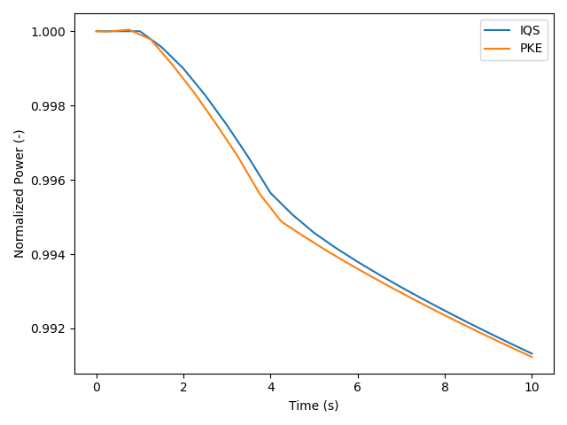
Figure 3: Comparison of normalized power between the IQS and PKE methods with the same reactivity profile imposed.

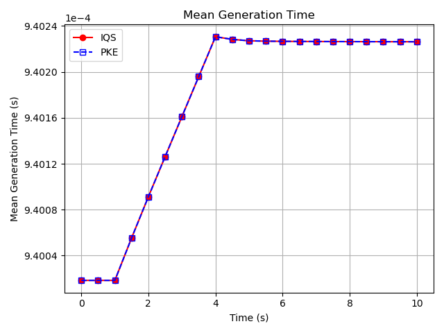
Comparison of mean generation time ($\Lambda$) between the IQS and PKE transient results.

Figure 4: Comparison of mean generation time ( $var element = document.getElementById("moose-equation-0c994679-2249-484c-86fc-1260f862b391");katex.render("\\Lambda", element, {displayMode:false,throwOnError:false});$ ) between the IQS and PKE transient results.

Comparison of delayed neutron precursor fraction for the 0th group ($\beta_0$) between the IQS and PKE transient results.

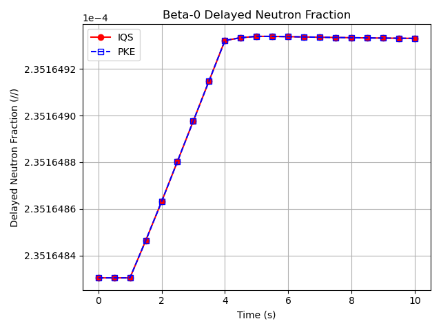
Figure 5: Comparison of delayed neutron precursor fraction for the 0th group ( $var element = document.getElementById("moose-equation-ee225d33-9e0a-4d10-afd2-a45f00094d60");katex.render("\\beta_0", element, {displayMode:false,throwOnError:false});$ ) between the IQS and PKE transient results.

Comparison of delayed neutron precursor fraction for the 1st group ($\beta_1$) between the IQS and PKE transient results.

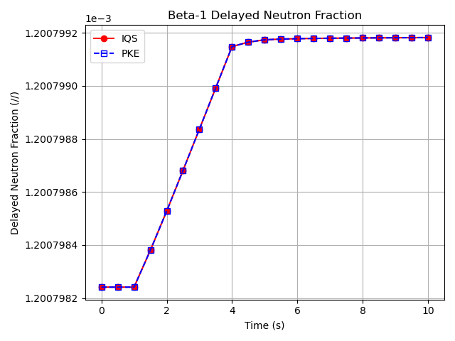
Figure 6: Comparison of delayed neutron precursor fraction for the 1st group ( $var element = document.getElementById("moose-equation-7229bd4c-b001-44c0-9c07-dba5b727616f");katex.render("\\beta_1", element, {displayMode:false,throwOnError:false});$ ) between the IQS and PKE transient results.

Comparison of delayed neutron precursor fraction for the 2nd group ($\beta_2$) between the IQS and PKE transient results.

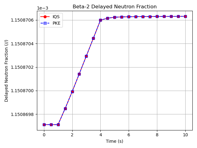
Figure 7: Comparison of delayed neutron precursor fraction for the 2nd group ( $var element = document.getElementById("moose-equation-f9740ecc-aab5-4f20-af99-05db428d7485");katex.render("\\beta_2", element, {displayMode:false,throwOnError:false});$ ) between the IQS and PKE transient results.

Comparison of delayed neutron precursor fraction for the 3rd group ($\beta_3$) between the IQS and PKE transient results.

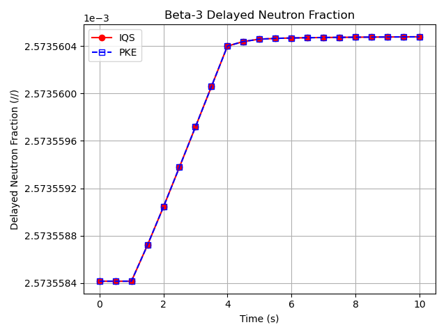
Figure 8: Comparison of delayed neutron precursor fraction for the 3rd group ( $var element = document.getElementById("moose-equation-2ce0ed74-22cb-42ce-8d38-3f8c2536e745");katex.render("\\beta_3", element, {displayMode:false,throwOnError:false});$ ) between the IQS and PKE transient results.

Comparison of delayed neutron precursor fraction for the 4th group ($\beta_4$) between the IQS and PKE transient results.

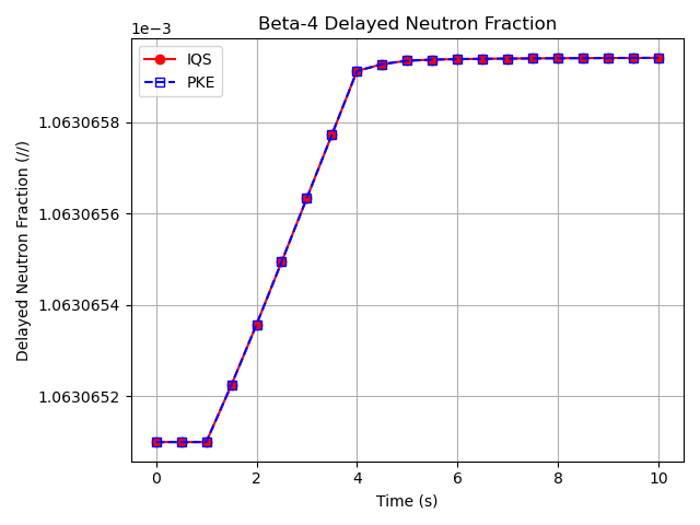
Figure 9: Comparison of delayed neutron precursor fraction for the 4th group ( $var element = document.getElementById("moose-equation-9044187c-3d99-4af0-8625-74f455150dad");katex.render("\\beta_4", element, {displayMode:false,throwOnError:false});$ ) between the IQS and PKE transient results.

Comparison of delayed neutron precursor fraction for the 5th group ($\beta_5$) between the IQS and PKE transient results.

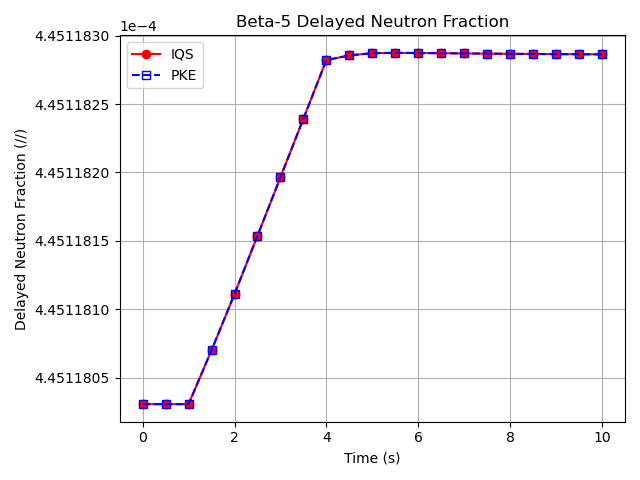
Figure 10: Comparison of delayed neutron precursor fraction for the 5th group ( $var element = document.getElementById("moose-equation-526d3a31-e6cc-4eba-9029-fa43e080c34a");katex.render("\\beta_5", element, {displayMode:false,throwOnError:false});$ ) between the IQS and PKE transient results.

Comparison of delayed neutron precursor decay constant for the 0th group ($\lambda_0$) between the IQS and PKE transient results.

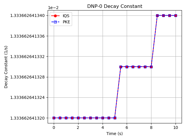
Figure 11: Comparison of delayed neutron precursor decay constant for the 0th group ( $var element = document.getElementById("moose-equation-8c13cc21-2804-47e8-b97e-3eaf3e0d0d2b");katex.render("\\lambda_0", element, {displayMode:false,throwOnError:false});$ ) between the IQS and PKE transient results.

Comparison of delayed neutron precursor decay constant for the 1st group ($\lambda_1$) between the IQS and PKE transient results.

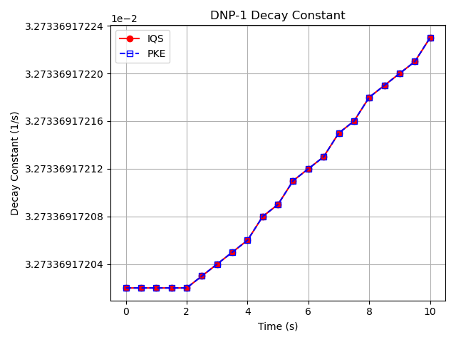
Figure 12: Comparison of delayed neutron precursor decay constant for the 1st group ( $var element = document.getElementById("moose-equation-57582c09-7c2d-4f31-813a-eea0a6bb87fc");katex.render("\\lambda_1", element, {displayMode:false,throwOnError:false});$ ) between the IQS and PKE transient results.

Comparison of delayed neutron precursor decay constant for the 2nd group ($\lambda_2$) between the IQS and PKE transient results.

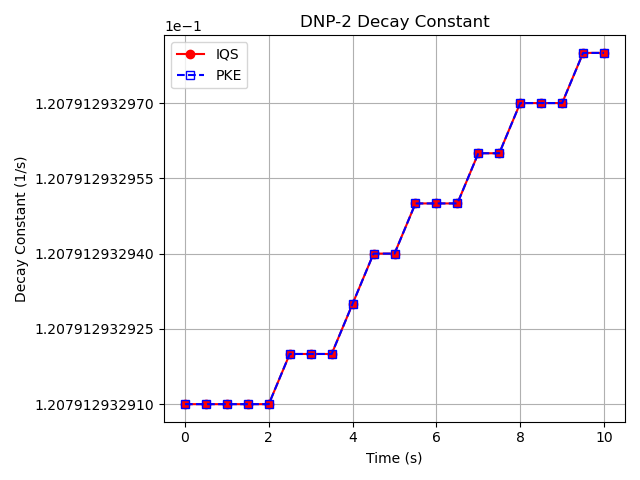
Figure 13: Comparison of delayed neutron precursor decay constant for the 2nd group ( $var element = document.getElementById("moose-equation-373ddbee-cf62-4b84-8081-5491bfe439c9");katex.render("\\lambda_2", element, {displayMode:false,throwOnError:false});$ ) between the IQS and PKE transient results.

Comparison of delayed neutron precursor decay constant for the 3rd group ($\lambda_3$) between the IQS and PKE transient results.

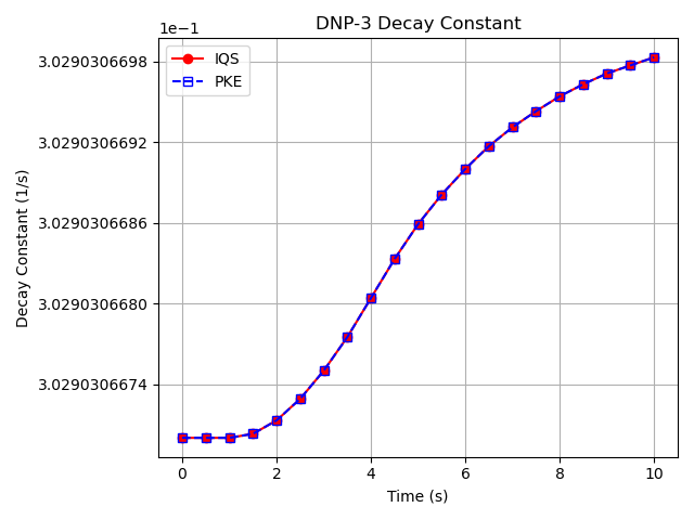
Figure 14: Comparison of delayed neutron precursor decay constant for the 3rd group ( $var element = document.getElementById("moose-equation-ef898a09-4b21-4010-96a0-109263c01c50");katex.render("\\lambda_3", element, {displayMode:false,throwOnError:false});$ ) between the IQS and PKE transient results.

Comparison of delayed neutron precursor decay constant for the 4th group ($\lambda$_4) between the IQS and PKE transient results.

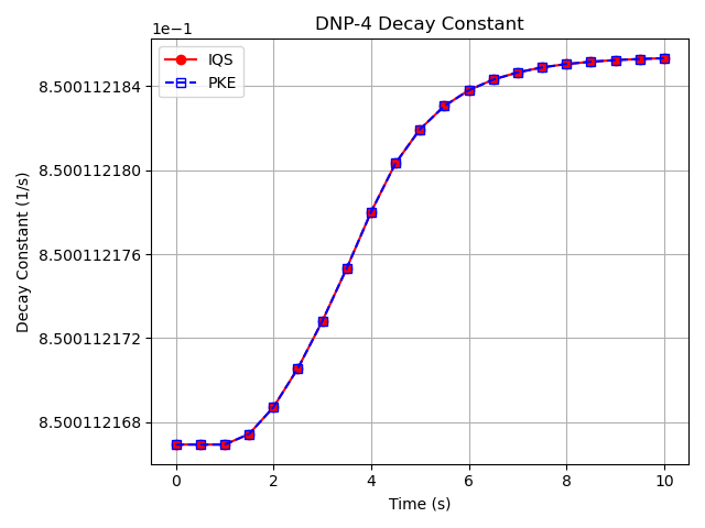
Figure 15: Comparison of delayed neutron precursor decay constant for the 4th group ( $var element = document.getElementById("moose-equation-e4c9afae-678f-4c30-978b-70b6936be53a");katex.render("\\lambda", element, {displayMode:false,throwOnError:false});$ _4) between the IQS and PKE transient results.

Comparison of delayed neutron precursor decay constant for the 5th group ($\lambda_5$) between the IQS and PKE transient results.

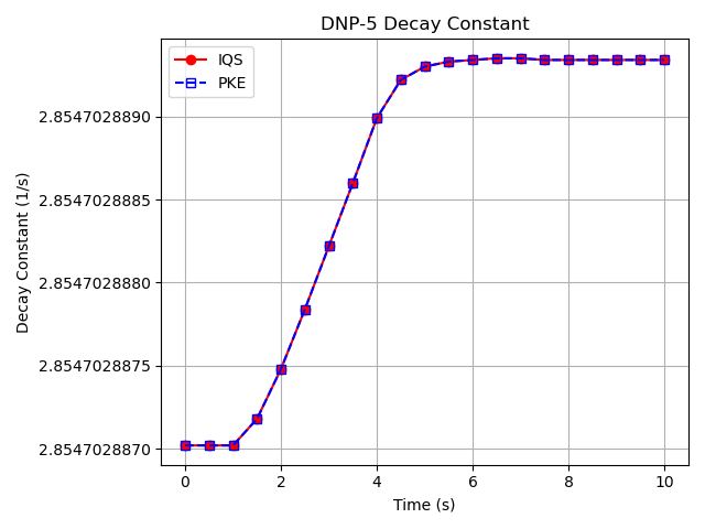
Figure 16: Comparison of delayed neutron precursor decay constant for the 5th group ( $var element = document.getElementById("moose-equation-611a7b99-2c8e-44a3-8887-f19b96f0e054");katex.render("\\lambda_5", element, {displayMode:false,throwOnError:false});$ ) between the IQS and PKE transient results.

Comparison of delayed neutron precursor concentration for the 0th group ($C_0$) between the IQS and PKE transient results.

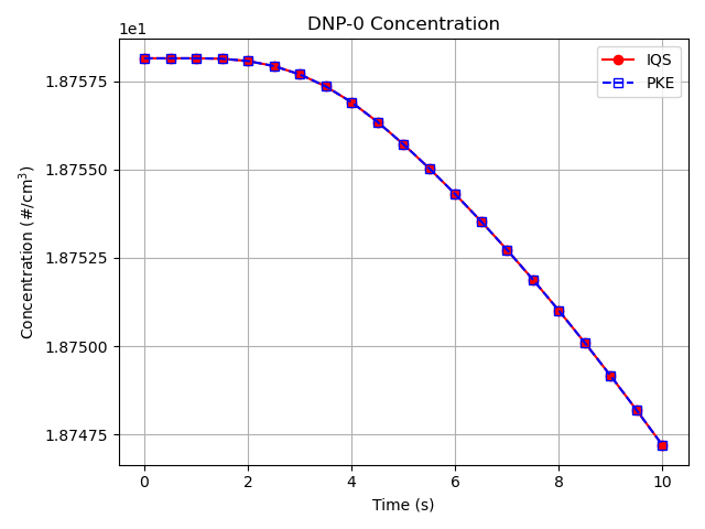
Figure 17: Comparison of delayed neutron precursor concentration for the 0th group ( $var element = document.getElementById("moose-equation-e15af618-5273-4675-8815-bc066dcc2f69");katex.render("C_0", element, {displayMode:false,throwOnError:false});$ ) between the IQS and PKE transient results.

Comparison of delayed neutron precursor concentration for the 1st group ($C_1$) between the IQS and PKE transient results.

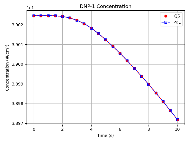
Figure 18: Comparison of delayed neutron precursor concentration for the 1st group ( $var element = document.getElementById("moose-equation-c1b680c6-d78a-4e87-88ff-dc985b721da4");katex.render("C_1", element, {displayMode:false,throwOnError:false});$ ) between the IQS and PKE transient results.

Comparison of delayed neutron precursor concentration for the 2nd group ($C_2$) between the IQS and PKE transient results.

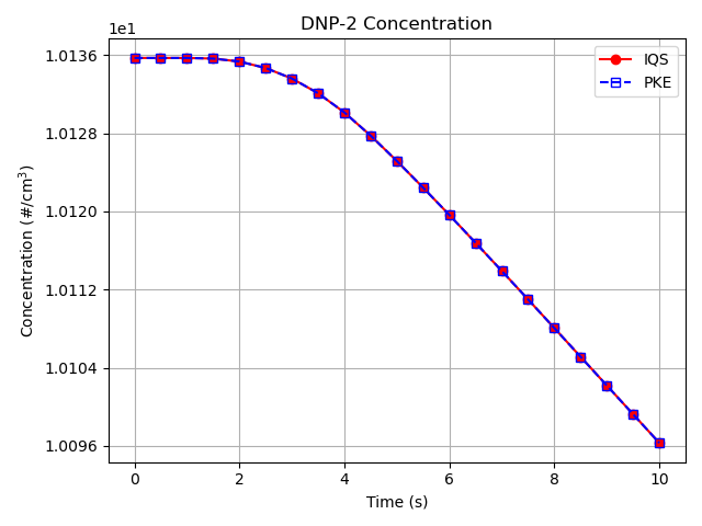
Figure 19: Comparison of delayed neutron precursor concentration for the 2nd group ( $var element = document.getElementById("moose-equation-8e278e83-6ae4-448d-a285-6449260d222b");katex.render("C_2", element, {displayMode:false,throwOnError:false});$ ) between the IQS and PKE transient results.

Comparison of delayed neutron precursor concentration for the 3rd group ($C_3$) between the IQS and PKE transient results.

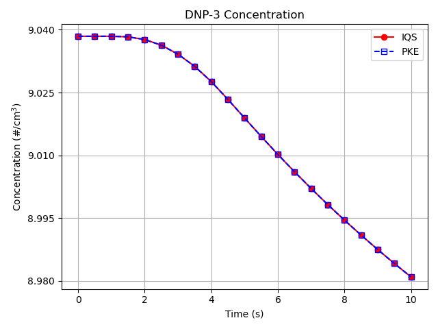
Figure 20: Comparison of delayed neutron precursor concentration for the 3rd group ( $var element = document.getElementById("moose-equation-b53b2e04-5b18-4ec4-a6ae-a434ef840f28");katex.render("C_3", element, {displayMode:false,throwOnError:false});$ ) between the IQS and PKE transient results.

Comparison of delayed neutron precursor concentration for the 4th group ($C_4$) between the IQS and PKE transient results.

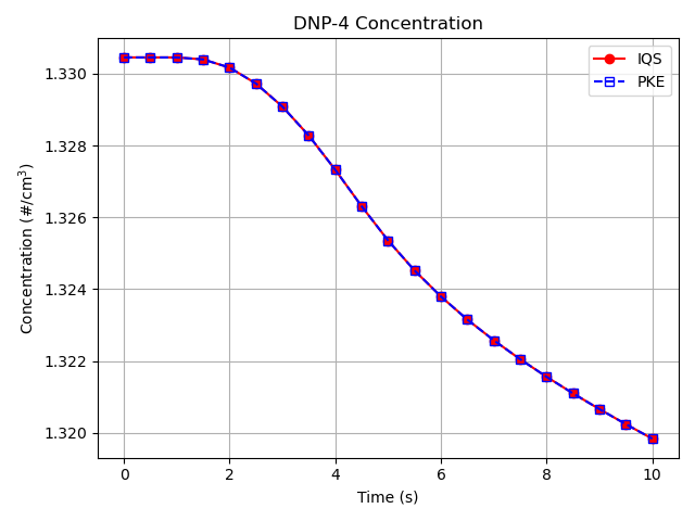
Figure 21: Comparison of delayed neutron precursor concentration for the 4th group ( $var element = document.getElementById("moose-equation-e55da3d7-ca68-4889-afdd-3c62d7832931");katex.render("C_4", element, {displayMode:false,throwOnError:false});$ ) between the IQS and PKE transient results.

Comparison of delayed neutron precursor concentration for the 5th group ($C_5$) between the IQS and PKE transient results.

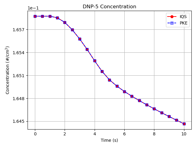
Figure 22: Comparison of delayed neutron precursor concentration for the 5th group ( $var element = document.getElementById("moose-equation-44148b31-f3c9-4c86-a726-7144e509f068");katex.render("C_5", element, {displayMode:false,throwOnError:false});$ ) between the IQS and PKE transient results.

References

R. Stewart, P. Balestra, D. Reger, and E. Merzari. Generation of localized reactor point kinetics parameters using coupled neutronic and thermal fluid models for pebble-bed reactor transient analysis. Annals of Nuclear Energy, 174:109143, 2022. URL: https://www.sciencedirect.com/science/article/pii/S0306454922001785#s0065, doi:https://doi.org/10.1016/j.anucene.2022.109143.

@article{Stewart2022,
    author = "Stewart, R. and Balestra, P. and Reger, D. and Merzari, E.",
    title = "Generation of localized reactor point kinetics parameters using coupled neutronic and thermal fluid models for pebble-bed reactor transient analysis",
    journal = "Annals of Nuclear Energy",
    volume = "174",
    pages = "109143",
    year = "2022",
    issn = "0306-4549",
    doi = "https://doi.org/10.1016/j.anucene.2022.109143",
    url = "https://www.sciencedirect.com/science/article/pii/S0306454922001785\#s0065",
    keywords = "Pebble-bed reactor, Multiphysics transient, Local reactivity coefficients, Point kinetics parameters"
}

Steady - State Results
PKE Parameters and Reactivity Coefficients
Transient Results
References