Simulations with a groove profile
Realistic surface wear profiles are inherently complex, and obtaining such data from the public domain can be challenging. In this study, these defects are idealized as grooves, as illustrated in the accompanying Figure 1.
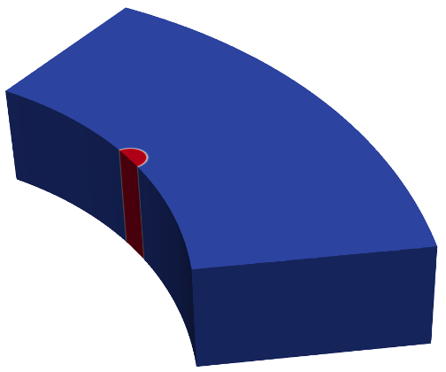
Figure 1: Schematic illustrating the wear profile idealized as a groove on the surface of the reflector block.
Computational Model Description
Figure 2 shows the refined mesh for the reflector block. The mesh is finely refined at the center to capture the stress concentrations due to the groove.
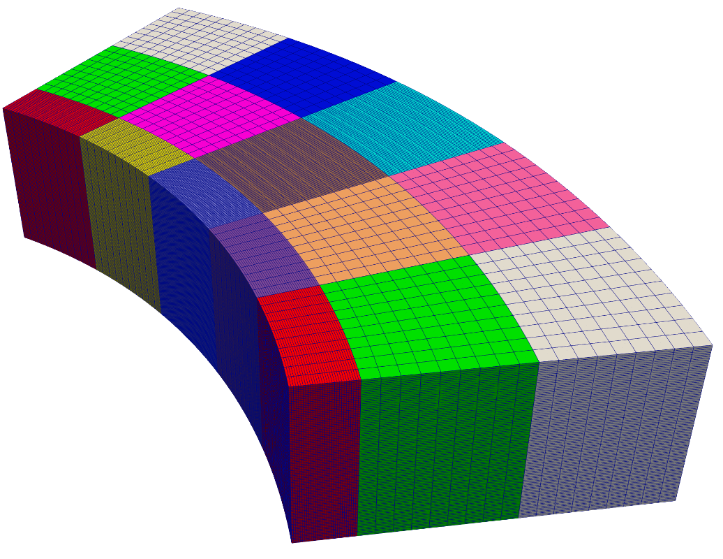
Figure 2: Refined mesh of a reflector block.
# ==============================================================================
# 3D stress analysis of a graphite reflector block with a groove
# Application : Grizzly
# ------------------------------------------------------------------------------
# Idaho Falls, INL, 2024
# Author(s): Ben Spencer, Will Hoffman
# If using or referring to this model, please cite as explained on
# https://mooseframework.inl.gov/virtual_test_bed/citing.html
# ==============================================================================

sector_angle = '${fparse 51*pi/180}'

radius_wear = 0.05 #m
interface_width = '${fparse radius_wear/5}' #m

delta_center_radius = 0.0 # how much do you want to move the center away from the surface #m

# endtime = 1892160000 #s
dt_max = 5e6 #s

Tmax_A1 = -36.406902443685375
Tmax_B1 = 899.4907346560636
Tmax_z01 = 0.5788213284387279
Tmin_A2 = -30.744024831884484
Tmin_B2 = 899.8512009151575
Tmin_z02 = 0.591661495195294
x0c = 1.2 #m
thickness = 0.6 #m

B_flux = -11.7708550271939
x0v = 1.26
Fmax_a = 1.264e+15
Fmax_b = -1.260e+16
Fmax_c = 3.202e+16
Fmax_d = -1.887e+15

#SpecifiedSmoothCircleIC Parameters
R_i = 1.2 #m
x_coord = '${fparse (R_i-delta_center_radius)*cos(0.5*sector_angle)}'  #m
y_coord = '${fparse (R_i-delta_center_radius)*sin(0.5*sector_angle)}'  #m
#z_coord = 1.76 #m

[GlobalParams]
  displacements = 'disp_x disp_y disp_z'
[]

[Mesh]
  type = FileMesh
  file = '../2_pit/FineMesh_Wear_Baseline.e'
[]

[Physics]

  [SolidMechanics]

    [QuasiStatic]
      [all]
        add_variables = true
        strain = FINITE
        automatic_eigenstrain_names = true
        generate_output = 'stress_xx stress_xy stress_xz stress_yy stress_yx stress_yz stress_zz stress_zx stress_zy
                      vonmises_stress max_principal_stress mid_principal_stress min_principal_stress
                      strain_xx strain_yy strain_zz elastic_strain_xx elastic_strain_yy elastic_strain_zz'
      []
    []
  []
[]

# Functions for temperature and fluence (flux * t)
[Functions]
  # Parsed function for temperature
  [T_func]
    type = ParsedFunction
    expression = 'r := (x^2 + y^2)^0.5;
             Tmax := ${Tmax_A1}*cos(z-${Tmax_z01}) + ${Tmax_B1};
             Tmin := ${Tmin_A2}*cos(z-${Tmin_z02}) + ${Tmin_B2};
             Tmax - (Tmax-Tmin)*(r-${x0c})/${thickness}'
  []

  # Fluence function (flux * time) using y #n/m^2
  [fluence_func]
    type = ParsedFunction
    expression = 'r := (x^2 + y^2)^0.5;
             Fmax := ${Fmax_a}*z^3 + ${Fmax_b}*z^2 + ${Fmax_c}*z + ${Fmax_d};
             Fmax*exp(${B_flux}*(r-${x0v}))*t'
  []
  [groove]
    type = ParsedFunction
    expression = 'r := ((x-${x_coord})^2 + (y-${y_coord})^2)^0.5;
                  int_factor := exp(-8*(r-${radius_wear})/${interface_width});
                  int_factor/(1 + int_factor)'
  []
[]

# AuxVariables for temperature and fluence
[AuxVariables]
  [temperature]
  []
  [volume]
    order = CONSTANT
    family = MONOMIAL
  []
  [eta]
  []
[]

# AuxKernels to assign the temperature and fluence functions
[AuxKernels]
  [T_aux]
    type = FunctionAux
    variable = temperature
    function = T_func
    execute_on = initial
  []
  [volume_aux]
    type = VolumeAux
    variable = volume
  []
[]

[ICs]
  [eta_ic]
    type = FunctionIC
    variable = eta
    function = groove
  []
[]

# Materials
[Materials]

  [h_void]
    type = SwitchingFunctionMaterial
    eta = eta
    h_order = HIGH
    function_name = h_void
    output_properties = 'h_void'
    # outputs = exodus
  []

  [h_mat]
    type = DerivativeParsedMaterial
    expression = '1-h_void'
    coupled_variables = 'eta'
    property_name = h_mat
    material_property_names = 'h_void'
    # outputs = exodus
  []

  [elastic_tensor_matrix]
    type = ComputeIsotropicElasticityTensor
    youngs_modulus = 10.3e9 #Pa
    poissons_ratio = 0.14
    base_name = Cijkl_matrix
  []

  [elastic_tensor_void]
    type = ComputeIsotropicElasticityTensor
    youngs_modulus = 1e-3 #Pa
    poissons_ratio = 1e-3
    base_name = Cijkl_void
  []

  [elasticity_tensor]
    type = CompositeElasticityTensor
    tensors = 'Cijkl_matrix Cijkl_void'
    weights = 'h_mat            h_void'
    coupled_variables = 'eta'
  []

  [neutron_fluence]
    type = GenericFunctionMaterial
    prop_names = fast_neutron_fluence
    prop_values = fluence_func
    # outputs = exodus
  []

  [thermal]
    type = HeatConductionMaterial
    thermal_conductivity = 63 #W/mK
    specific_heat = 1502 #J/KgK
  []
  [density]
    type = GenericConstantMaterial
    prop_names = 'density'
    prop_values = 1774.0 #Kg/m^3
  []

  [thermal_expansion]
    type = StructuralGraphiteThermalExpansionEigenstrain
    eigenstrain_name = thermal_expansion
    graphite_grade = IG_110
    stress_free_temperature = 300.0 #K
    fluence_conversion_factor = 1.0
    temperature = temperature
    # outputs = exodus
  []
  [GraphiteGrade_creep]
    type = StructuralGraphiteCreepUpdate
    fluence_conversion_factor = 1.0
    graphite_grade = IG_110
    temperature = temperature
    creep_scale_factor = 1.0
    # outputs = exodus
  []

  [graphite_irrad_strain]
    type = StructuralGraphiteIrradiationEigenstrain
    temperature = temperature
    graphite_grade = IG_110
    fluence_conversion_factor = 1.0
    eigenstrain_name = irrad_strain
    # outputs = exodus
  []

  [stress]
    type = ComputeMultipleInelasticStress
    inelastic_models = 'GraphiteGrade_creep'
  []
[]

# BCs
[BCs]
  [x_fixed]
    type = DirichletBC
    preset = true
    variable = disp_x
    value = 0
    boundary = 'fixed'
  []
  [y_fixed]
    type = DirichletBC
    preset = true
    variable = disp_y
    value = 0
    boundary = 'fixed y_z_roller y_roller'
  []
  [z_fixed]
    type = DirichletBC
    preset = true
    variable = disp_z
    value = 0
    boundary = 'fixed y_z_roller'
  []
[]

[VectorPostprocessors]
  # [auxvars]
  #   type = ElementValueSampler
  #   sort_by = id
  #   variable = 'volume max_principal_stress mid_principal_stress min_principal_stress'
  #   execute_on = 'timestep_end'
  # []
  [line]
    type = LineValueSampler
    start_point = '1.0914 0.5215 1.76'
    end_point = '1.6146 0.7715 1.76'
    num_points = 100
    sort_by = 'x'
    variable = 'disp_x disp_y disp_z temperature eta'
    execute_on = timestep_end
  []
[]

# Executioner
[Executioner]
  type = Transient
  solve_type = 'NEWTON'
  petsc_options_iname = '-pc_type -pc_hypre_type -pc_hypre_boomeramg_strong_threshold'
  petsc_options_value = 'hypre    boomeramg      0.6'
  line_search = 'none'
  # end_time = ${endtime}
  num_steps = 1
  dtmax = ${dt_max}
  nl_abs_tol = 1.0e-08
  nl_rel_tol = 1.0e-10
  nl_max_its = 15
  l_max_its = 50
  [TimeStepper]
    type = IterationAdaptiveDT
    dt = 1 #s
    growth_factor = 3.0
    cutback_factor = 0.5
  []
  [Predictor]
    type = SimplePredictor
    scale = 1.0
  []
[]

# Outputs
[Outputs]
  sync_times = '0 315360000 630720000 946080000 1261440000 1576800000 1892160000'

  # [exodus]
  #   type = Exodus
  #   #sync_only = true
  # []

  [csv]
    type = CSV
    execute_vector_postprocessors_on = FINAL
    # sync_only = true
  []
  checkpoint = false
[]The model setup adheres closely to the input file description provided in the Baseline simulation with combined thermal and radiation effects. The additional steps involve the initialization of the groove and the configuration of the elasticity tensor, which are detailed below.
Initialization of the groove profile
In structural analysis, a groove acts as a stress concentrator. Assigning appropriate elastic properties to the groove is crucial for accurately capturing this effect. In this model, the groove is not explicitly represented. Instead, near-zero elastic properties are assigned to the groove region. This approach ensures that the stress concentration effects are appropriately accounted for without the need for detailed groove geometry.
The following block defines a variable eta which is 1 within the groove and 0 elsewhere, with a smooth transition between these regions.
[ICs]
  [eta_ic]
    type = FunctionIC
    variable = eta
    function = groove
  []
[]Configuration of the elasticity tensor
The following blocks define the material properties and elasticity tensors based on the variable eta.
[Materials]

  [h_void]
    type = SwitchingFunctionMaterial
    eta = eta
    h_order = HIGH
    function_name = h_void
    output_properties = 'h_void'
    # outputs = exodus
  []

  [h_mat]
    type = DerivativeParsedMaterial
    expression = '1-h_void'
    coupled_variables = 'eta'
    property_name = h_mat
    material_property_names = 'h_void'
    # outputs = exodus
  []

  [elastic_tensor_matrix]
    type = ComputeIsotropicElasticityTensor
    youngs_modulus = 10.3e9 #Pa
    poissons_ratio = 0.14
    base_name = Cijkl_matrix
  []

  [elastic_tensor_void]
    type = ComputeIsotropicElasticityTensor
    youngs_modulus = 1e-3 #Pa
    poissons_ratio = 1e-3
    base_name = Cijkl_void
  []

  [elasticity_tensor]
    type = CompositeElasticityTensor
    tensors = 'Cijkl_matrix Cijkl_void'
    weights = 'h_mat            h_void'
    coupled_variables = 'eta'
  []

  [neutron_fluence]
    type = GenericFunctionMaterial
    prop_names = fast_neutron_fluence
    prop_values = fluence_func
    # outputs = exodus
  []

  [thermal]
    type = HeatConductionMaterial
    thermal_conductivity = 63 #W/mK
    specific_heat = 1502 #J/KgK
  []
  [density]
    type = GenericConstantMaterial
    prop_names = 'density'
    prop_values = 1774.0 #Kg/m^3
  []

  [thermal_expansion]
    type = StructuralGraphiteThermalExpansionEigenstrain
    eigenstrain_name = thermal_expansion
    graphite_grade = IG_110
    stress_free_temperature = 300.0 #K
    fluence_conversion_factor = 1.0
    temperature = temperature
    # outputs = exodus
  []
  [GraphiteGrade_creep]
    type = StructuralGraphiteCreepUpdate
    fluence_conversion_factor = 1.0
    graphite_grade = IG_110
    temperature = temperature
    creep_scale_factor = 1.0
    # outputs = exodus
  []

  [graphite_irrad_strain]
    type = StructuralGraphiteIrradiationEigenstrain
    temperature = temperature
    graphite_grade = IG_110
    fluence_conversion_factor = 1.0
    eigenstrain_name = irrad_strain
    # outputs = exodus
  []

  [stress]
    type = ComputeMultipleInelasticStress
    inelastic_models = 'GraphiteGrade_creep'
  []
[]The h_void block defines a switching function material for eta, producing the property h_void. The h_mat block calculates the complementary property h_mat as 1 - h_void. The elastic_tensor_matrix block defines the elasticity tensor for the matrix material with a specified Young's modulus and Poisson's ratio. The elastic_tensor_void block defines the elasticity tensor for the void (groove) with very low elastic properties. Finally, the elasticity_tensor block creates a composite elasticity tensor by combining matrix and void properties, weighted by h_mat and h_void, respectively.
Running the model
To run this model using the Grizzly executable, run the following command:
mpiexec -n 300 /path/to/app/grizzly-opt -i groove_r0p05.i
Note: HPC resources were used to perform this simulation
The following Exodus results file will be produced: groove_r0p05_exodus.e
The Exodus output file can be visualized with Paraview.
Results
Figure 3 presents the distribution of maximum principal stress (MPa) at 40 years for the reflector block with dimensions 0.6 m (radial), 0.305 m (axial), and 1.55 m (azimuthal span at 51°), evaluated at a cross-section corresponding to the location of maximum stress. The baseline configuration is compared with models containing pit and groove-type surface defects of radii 0.01 m and 0.05 m. The results show that groove defects cause noticeably higher stress concentrations than pit defects, with the largest groove producing a peak stress of about 18 MPa, approximately a 62 % increase over the baseline.
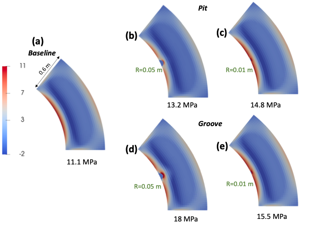
Figure 3: Distribution of maximum principal stress (MPa) at 40 years for (a) the baseline case at a cross-section corresponding to the location of maximum stress, (b) baseline case with a pit of radius 0.05 m, (c) baseline case with a pit of radius 0.01 m, (d) baseline case with a groove of radius 0.05 m, and (e) baseline case with a groove of radius 0.01 m.