Creation of infiltration profiles
Given that the pore sizes in nuclear graphite material are several orders of magnitude smaller than the actual component, resolving the pore structure is impractical. Therefore, the graphite component is modeled as a continuum. Within this constraint, initializing the infiltration profile is not straightforward. To address this, a diffusion equation, similar to a porous flow model, is employed to establish a physically realistic infiltration profile before proceeding with the stress analysis.
Computational Model Description
Figure 1 shows the mesh of the unit cell of the MSRE graphite stringer.
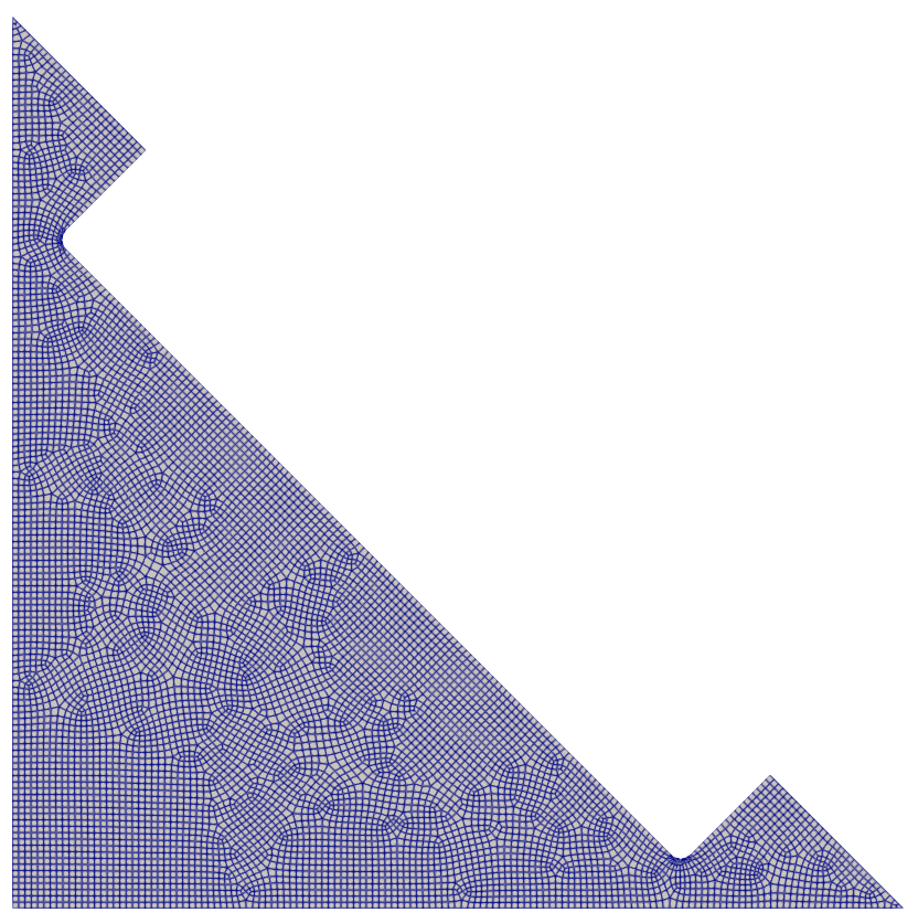
Figure 1: Finite element mesh of the 2D unit cell of the graphite stringer.
Files used by this model include:
MOOSE input file
Exodus mesh file
This document reviews the basic elements of the input file, listed in full here:
# ==============================================================================
# Generation of 2D Molten Salt Infiltration Profiles in Graphite
# Application : MOOSE
# ------------------------------------------------------------------------------
# Idaho Falls, INL, 2025
# Author(s): V Prithivirajan, Ben Spencer
# If using or referring to this model, please cite as explained on
# https://mooseframework.inl.gov/virtual_test_bed/citing.html
# ==============================================================================

# The diffusion field profile is smooth and continuous, but for this problem
# we need a binary field (infiltrated vs. no infiltration), mimicking the physical behavior.
# The threshold value converts the continuous field to a binary field.

threshold = 0.8

# vol_frac_threshold represents the infiltration volume fraction
vol_frac_threshold = 0.30

#Diffusivity constant
diffusivity = 1e-3 # m^2/s

[Mesh]
  # 2D msre mesh file (saved as a gold file for convenience)
  file = 'gold/2D_CreateInfiltrationProfile_out.e'
[]

#diffusion field variable, representing the salt infiltration
[Variables]
  [diffused]
    order = FIRST
    family = LAGRANGE
  []
[]

#smooth is a binary variable, obtained by penalizing diffused variable
[AuxVariables]
  [smooth]
    order = FIRST
    family = LAGRANGE
  []
[]

# Governing equation for diffusion
[Kernels]
  [diff]
    type = MatDiffusion
    variable = diffused
    diffusivity = ${diffusivity}
  []
  [timederivative]
    type = TimeDerivative
    variable = diffused
  []
[]

[AuxKernels]
  [smoothAux]
    type = ParsedAux
    coupled_variables = 'diffused'
    variable = smooth
    expression = 'diffused>=${threshold}'
  []
[]

# terminate stops the simulation when the desired volume fraction is reached
[UserObjects]
  [terminate]
    type = Terminator
    expression = 'elemavg >= ${vol_frac_threshold}'
    fail_mode = HARD
  []
[]

[Postprocessors]
  [elemavg]
    type = ElementAverageValue
    variable = smooth
    execute_on = 'initial timestep_end'
  []
[]

# Boundary condition
[BCs]
  [conc]
    type = DirichletBC
    variable = diffused
    boundary = 'right_channelboundary'
    value = 1
  []
[]

# Solver settings
[Executioner]
  type = Transient

  solve_type = 'NEWTON'
  petsc_options_iname = '-pc_type -pc_hypre_type -pc_hypre_boomeramg_strong_threshold'
  petsc_options_value = 'hypre    boomeramg      0.6'

  dt = 0.005   #s
  end_time = 1 #s
[]

# Outputs
[Outputs]
  exodus = true
[]Global Variables
These are input parameters defined in the global scope, so they could be accessed by any object within the MOOSE input file. These streamline the workflows.
# The diffusion field profile is smooth and continuous, but for this problem
# we need a binary field (infiltrated vs. no infiltration), mimicking the physical behavior.
# The threshold value converts the continuous field to a binary field.

threshold = 0.8

# vol_frac_threshold represents the infiltration volume fraction
vol_frac_threshold = 0.30

#Diffusivity constant
diffusivity = 1e-3 # m^2/s

[Mesh]
Mesh
This block defines the finite element mesh that will be used. In this case, the mesh is read from a file in the Exodus (.e) format. The mesh for this problem was created using Cubit. The journal file to generate the mesh can be found in the following link: Models for Infiltration effects on graphite behavior.
[Mesh]
  # 2D msre mesh file (saved as a gold file for convenience)
  file = 'gold/2D_CreateInfiltrationProfile_out.e'
[]Variables
This block defines the field variables that will be solved for in the nonlinear equation system. In this model, the only variable defined in this step.
[Variables]
  [diffused]
    order = FIRST
    family = LAGRANGE
  []
[]AuxVariables
This block defines AuxVariables (i.e., auxiliary variables), which are field variables that are not part of the system of equations being solved. In this case, it is a binary variable, obtained by penalizing the diffused variable
[AuxVariables]
  [smooth]
    order = FIRST
    family = LAGRANGE
  []
[]Kernels
This block defines the terms in the partial differential equations for the physics being modeled. In this case, the transient diffusion equation consisting of the time derivative term and the Laplacian terms are defined.
[Kernels]
  [diff]
    type = MatDiffusion
    variable = diffused
    diffusivity = ${diffusivity}
  []
  [timederivative]
    type = TimeDerivative
    variable = diffused
  []
[]AuxKernels
This block defines the models that compute the values stored in the AuxVariables that were previously defined. In this case, these are objects that binarizes the diffused variable.
[AuxKernels]
  [smoothAux]
    type = ParsedAux
    coupled_variables = 'diffused'
    variable = smooth
    expression = 'diffused>=${threshold}'
  []
[]UserObjects
This block defines the custom objects that perform specific tasks within the MOOSE framework. In this case, we use the Terminator user-object to stop the simulation after the infiltration amount reaches the user input, vol_frac_threshold.
[UserObjects]
  [terminate]
    type = Terminator
    expression = 'elemavg >= ${vol_frac_threshold}'
    fail_mode = HARD
  []
[]Postprocessors
This block is used to defined to calculate specific items of interest to the user. In this case, the infiltration amount is calculated and printed to the screen as well as output to a CSV file.
[Postprocessors]
  [elemavg]
    type = ElementAverageValue
    variable = smooth
    execute_on = 'initial timestep_end'
  []
[]BCs
The boundary conditions are defined in this block. For this case, the salt-facing graphite channel is prescribed with a Dirichlet BC for the diffused variable to be unity. The rest of the surfaces will automatically be assigned as Neumann BCs, meaning the flux will be zero.
[BCs]
  [conc]
    type = DirichletBC
    variable = diffused
    boundary = 'right_channelboundary'
    value = 1
  []
[]Executioner
The parameters in this block control the solution strategy used, convergence tolerances, time increment and end time, and other relevant settings.
[Executioner]
  type = Transient

  solve_type = 'NEWTON'
  petsc_options_iname = '-pc_type -pc_hypre_type -pc_hypre_boomeramg_strong_threshold'
  petsc_options_value = 'hypre    boomeramg      0.6'

  dt = 0.005 #s
  end_time = 1 #s
[]Outputs
This block defines the types of output that are generated. The CSV outputs the amount of infiltration at various time steps to a file for postprocessing. The Exodus output is primarily used for inspection of the results.
[Outputs]
  exodus = true
[]Running the model
To run this model using the MOOSE executable with the combined module, use the following command:
mpiexec -n 8 /path/to/app/combined-opt -i 2D_CreateInfiltrationProfile.i
The following output files will be produced:
The Exodus results file:
2D_CreateInfiltrationProfile_exodus.eThe CSV results file:
2D_CreateInfiltrationProfile_csv.csv
The Exodus output file can be visualized with Paraview.