LMCR Primary Loop nekRS LES Model
Contact: Jun Fang, fangj.at.anl.gov
Model link: LMCR nekRS LES Model
The CFD solver nekRS is not included in the VTB continuous integration test suite at this time. Users are encouraged to reach out to the nekRS developer team at Argonne by emailing the POC (Jun Fang at [email protected]). Additionally, a beta version of the nekRS tutorial is available at the nekRS Documentation.
Model Overview
The LOTUS Molten Chloride Reactor (LMCR) is an open-core, fast-spectrum, liquid-fueled molten salt reactor concept that circulates chloride fuel salt through the reactor vessel and primary loop. The fuel salt, represented here by a UCl-NaCl eutectic mixture, provides both the fissile material and the primary heat-transfer medium (Walter et al., 2022; Tano et al., 2023). The high-fidelity computational fluid dynamics (CFD) model documented on this page represents an MCRE-like LMCR primary-loop configuration in which the unmoderated core cavity is connected to a curved inlet pipe, outlet pipe, pump region, and heat-exchanger leg. The checked-in nekRS case name is mcre, so the run files retain that historical name even though this VTB page documents the LMCR primary-loop LES benchmark.
Because fission energy is deposited directly into the circulating fuel, the flow field controls more than pressure drop and heat removal. It also affects delayed neutron precursor residence time, spatial reactivity feedback, and the temperature field seen by lower-fidelity multiphysics models. Although reactor conceptual designs may include a bottom inlet grid or flow-straightening component to distribute and homogenize core flow, this component was intentionally omitted from the present CFD model to maintain a simplified geometry. As a result, without internal structures to homogenize the incoming jet in the open cavity, centrifugal acceleration from the upstream elbow drives the inlet stream toward the vessel wall, producing strongly three-dimensional recirculation, large coherent eddies, and persistent short-circuiting paths between the inlet and outlet.
This nekRS model is intended to generate high-resolution large-eddy simulation (LES) data for understanding the LMCR primary-loop hydrodynamics and for calibrating engineering-scale thermal-hydraulic tools such as Pronghorn. The current checked-in case solves the incompressible isothermal flow problem with the temperature equation disabled, so the documented fields focus on velocity magnitude and the vertical velocity component. Accordingly, this study is centered on the loop flow velocity distribution and its turbulence characteristics.
The case files are stored in msr/lotus/les. The checked-in mcre.par file is a demonstration template. To speed up start-up and develop the turbulent state more quickly, you should begin runs with a lower polynomial order (for example or ) and a reduced Reynolds number. After the transient has developed, set the non-dimensional viscosity to 1/10742.82 and restart at a higher polynomial order (for example ) to run the long-averaging production calculation.
System Specifications
Table 1 summarizes the primary design and material properties used for the high-fidelity LES setup. The operating point corresponds to a low-power molten chloride fuel loop at 900 K.
Table 1: Representative LMCR operating conditions and fuel-salt properties for the nekRS LES model.
| Parameter | Value |
|---|---|
| Core power | 100.0 kW |
| Operating temperature | 900 K |
| Rated mass flow rate | 25 kg/s |
| Fuel salt composition | UCl (33.3 mol%) - NaCl (66.7 mol%) |
| U enrichment | 93.2 wt% |
| Density at 900 K | 3279.0 kg/m |
| Specific heat at 900 K | 640.0 J/(kg K) |
| Thermal conductivity at 900 K | 0.38 W/(m K) |
| Dynamic viscosity at 900 K | Pa s |
The reference core diameter is m. For the 25 kg/s operating point, the corresponding mean core flow speed is approximately 0.03883 m/s. The resulting core Reynolds number is
This Reynolds number is well above the laminar-to-turbulent transition range for internal flows and motivates the use of LES rather than a purely steady Reynolds-averaged Navier-Stokes (RANS) closure.
CFD Solver and Numerical Method
The flow is simulated with nekRS, a GPU-oriented spectral-element CFD solver for incompressible and low-Mach-number flows (Fischer et al., 2022). Like Nek5000, nekRS represents the solution in high-order hexahedral spectral elements, but it is implemented in C++ with OCCA backends for performance portability on GPU and CPU systems. This makes nekRS well suited for high-fidelity LES of the strongly swirling LMCR primary-loop flow.
The LES model uses the incompressible, constant-property form of the Navier-Stokes equations:
where is velocity, is pressure, is kinematic viscosity, and is the user-defined momentum source used to drive the loop. The checked-in case disables the scalar temperature solve because this stage of the benchmark is focused on hydrodynamic mixing, residence-time behavior, and velocity-field statistics.
The high-fidelity workflow uses lower-order transients to develop a turbulent initial condition before restarting at higher polynomial order (or higher resolution) for the production averaging run. Here, "production averaging" refers to the stage where, after initial numerical transients have washed out and the flow has reached a statistically stationary turbulent state, the simulation is continued over an extended physical duration to compute time-averaged statistics (such as mean velocity fields and turbulent fluctuations) used for engineering calibration and benchmarking. In the documented analysis, initial transients were developed with , while the final LES statistics targeting used for improved turbulent-scale resolution.
Case Setup
Input files
The nekRS case is named mcre. The main files are:
mcre.re2: spectral-element mesh in nekRS/Nek5000 format.mcre.co2: curved-side high-order geometry information.mcre.par: nekRS runtime parameters, solver tolerances, time-step controls, and material properties.mcre.usr: Nek-style user routines used for geometry scaling, boundary tag reconstruction, PID control, and the momentum-source calculation.mcre.udf: nekRS C++ user-defined functions that register and copy the body-force field to the device.planar.f: helper routine used to compute a planar average of velocity for flow-control feedback.
The primary nekRS settings are shown below.
[GENERAL]
polynomialOrder = 7
#startFrom =
stopAt = numSteps
numSteps = 10000

timeStepper = tombo2
#dt = 1.0e-6
#advectionSubCyclingSteps = 2
dt = targetCFL=4 + max=1e-2 + initial=1e-6

checkpointControl = steps
checkpointInterval = 1000

regularization = hpfrt + nModes=1 + scalingCoeff=20

[FLUID PRESSURE]
residualTol = 1e-04
initialGuess = projectionAconj+nVector=10

[FLUID VELOCITY]
boundaryTypeMap = W
rho = 1.0
viscosity = 1/10742.82
residualTol = 1e-06
The checked-in parameter file uses the second-order tombo2 (BDF2) time stepper, a target-CFL adaptive time step with a maximum nondimensional time step of , checkpoint output every 1,000 steps, pressure residual tolerance of , and velocity residual tolerance of . The hpfrt regularization option is enabled to stabilize under-resolved high-order content during turbulent transients.
Boundary conditions and geometry scaling
The case is nondimensionalized using the reference core diameter m as the characteristic length scale () and the nominal mean core flow speed m/s (from Table 1) as the characteristic velocity scale. Spatial scaling is applied in usrdat2, where each mesh coordinate is multiplied by to yield non-dimensional coordinates . The same routine reconstructs wall boundary tags from the mesh boundary IDs so that all solid surfaces use no-slip wall conditions.
      subroutine usrdat2

      include 'SIZE'
      include 'TOTAL'

      real Dhi
      n = nx1*ny1*nz1*nelt

C rescaled by the core diameter

      Dhi = 1.0/0.5
      call cmult(xm1,Dhi,n)
      call cmult(ym1,Dhi,n)
      call cmult(zm1,Dhi,n)

      ! reconstruct boundary tags
      do iel=1,nelv
      do ifc=1,2*ndim
         id_face = bc(5,ifc,iel,1)
         if (id_face.eq.2) then          ! wall faces
             cbc(ifc,iel,1) = 'W  '
             boundaryID(ifc,iel)=1
         else
             boundaryID(ifc,iel)=0
         endif
      enddo
      enddo

      return
      end
The velocity boundary-type map in mcre.par is W, so the flow is not driven by imposed inlet/outlet velocity conditions. Instead, the primary loop is circulated by a body force in the vertical pipe section. This approach avoids prescribing an artificial inlet profile immediately upstream of the open core and allows the loop flow to respond naturally to the curved pipe, expansion into the vessel, and outlet geometry.
Momentum-source flow control
A proportional-integral-derivative (PID) controller maintains the target mean core velocity. During userchk, the code computes a planar average of the vertical velocity across the core, compares it against the target nondimensional velocity of 1.0 (utar = 1.0), and updates the axial forcing term. Because the reference velocity is m/s, maintaining a non-dimensional core speed of ensures that the simulated flow corresponds to the physical 25 kg/s operating point. The force is applied in a selected vertical-pipe region and is saved periodically to pid_restart.dat so restarted simulations retain the controller history. The relevant user routine is included in the mcre.usr listing below.
      subroutine userchk

      include 'SIZE'
      include 'TOTAL'

      common /cforce/ forcx(lx1,ly1,lz1,lelv)
      common /pid_ctrl/ integral_error, prev_error, kp, ki, kd

      real norm(3), pt(3), ucore, planar_ave_m1
      real force, error, delt, utar
      real integral_error, derivative_error, prev_error
      real kp, ki, kd
      logical first_call, file_exists
      save first_call
      data first_call /.true./

      call nekrs_registerPtr('forcx', forcx)

C     Initialize PID parameters (tune these as needed)
      data kp /0.5/, ki /0.1/, kd /0.05/
      data integral_error /0.0/, prev_error /0.0/
      data delt /1.0/, utar /1.0/

C     Check if PID data file exists before reading
      if (first_call) then
         inquire(file='pid_restart.dat', exist=file_exists)
         if (file_exists) then
            open(unit=10, file='pid_restart.dat', status='old')
            read(10,*) kp, ki, kd, integral_error, prev_error
            close(10)
         endif
         first_call = .false.
      endif

C     return the pressure loss
      norm(1) = 1.0
      norm(2) = 0.0
      norm(3) = 0.0
      pt(1)   = 0.8
      pt(2)   = 0.0
      pt(3)   = 0.0
      ucore   = planar_ave_m1(vx,norm,pt,0.05)

C     PID Controller to adjust force
      error = utar - ucore
      integral_error = integral_error + error * delt
      derivative_error = (error - prev_error) / delt

      force = kp * error + ki * integral_error + kd * derivative_error

      prev_error = error

      if(nio.eq.0) then
         write(*,'(A, E12.4)') "ucore = ", ucore
         write(*,'(A, E12.4)') "error = ", error
         write(*,'(A, E12.4)') "force = ", force
         write(*,* )
      endif

C     compute the momentum source
      n = nx1*ny1*nz1*nelv

      do i = 1,n
        xx = xm1(i,1,1,1)
        yy = ym1(i,1,1,1)
        if(yy.gt.3.0) then
          if(xx.gt.-0.4.and.xx.lt.0.4) then
            forcx(i,1,1,1) = -force
          endif
        endif
      enddo

C     Save PID data to file for restart
      if (nio.eq.0 .and. mod(istep,10000).eq.0) then
         open(unit=11, file='pid_restart.dat', status='replace')
         write(11,*) kp, ki, kd, integral_error, prev_error
         close(11)
      endif

      return
      end
The force field is transferred from the Nek user routine to nekRS through mcre.udf. During setup (UDF_Setup), device memory is allocated and the initial force is evaluated from the velocity field. Every ten time steps during execution (UDF_ExecuteStep), nekRS copies the current solution to the Nek side, calls userchk, copies the updated forcx array into device memory, and applies it in userf via nrs->userSource as an explicit momentum source.
#ifdef __okl__

#endif

static deviceMemory<dfloat> o_nekFU;

void userf(double time)
{
  nrs->fluid->o_explicitTerms().copyFrom(o_nekFU, nrs->fluid->fieldOffsetSum);
}

/* UDF Functions */
void UDF_Setup()
{
  auto mesh = nrs->meshV;
  nrs->userSource = &userf;

  o_nekFU.resize(nrs->fluid->fieldOffsetSum);
  platform->linAlg->fill(nrs->fluid->fieldOffsetSum, 0.0, o_nekFU);

  double startTime = 0.0;
  platform->options.getArgs("START TIME", startTime);
  nrs->copyToNek(startTime, 0);
  nek::userchk();
  std::vector<dfloat> FUx(nek::ptr<double>("forcx"), nek::ptr<double>("forcx") + mesh->Nlocal);
  o_nekFU.copyFrom(FUx, mesh->Nlocal, 0 * nrs->fieldOffset);
}

void UDF_ExecuteStep(double time, int tstep)
{
  auto mesh = nrs->meshV;

  if (tstep % 10 == 0) {
    nrs->copyToNek(time, tstep);
    nek::userchk();
    std::vector<dfloat> FUx(nek::ptr<double>("forcx"), nek::ptr<double>("forcx") + mesh->Nlocal);
    o_nekFU.copyFrom(FUx, mesh->Nlocal, 0 * nrs->fieldOffset);
  }
}
Flow diagnostic plane
The planar average used by the PID controller is evaluated by planar.f. The helper routine integrates a user-provided field over a narrow band around the requested plane and restricts the diagnostic to the core region.
c-----------------------------------------------------------------------
      real function planar_ave_m1(phi,norm,pt,eps)
      implicit none
C
C     Compute area average of phi() on the
C     plane defined by normal 'norm' and point 'pt'
C
      include 'SIZE'
      include 'TOTAL'

      real phi(1),norm(3),pt(3),eps
      real aa,bb,cc,dd,w1,w2,x0,y0,z0,r0,rr,del,xsa,glsum

      integer i,j,k,n

      n=nx1*ny1*nz1*nelv

      aa=norm(1)
      bb=norm(2)
      cc=0.0
      if(if3d) cc=norm(3)
      dd=-1.0*(aa*pt(1)+bb*pt(2)+cc*pt(3))
      w1=0.0
      w2=0.0
      do i=1,n
        x0=xm1(i,1,1,1)
        y0=ym1(i,1,1,1)
        z0=zm1(i,1,1,1)
        IF(y0.lt.0.8) THEN !Here we consider only the MCRE core region
        r0=(aa*x0+bb*y0+cc*z0+dd)/sqrt(aa**2+bb**2+cc**2)
        rr=min(2.0,abs(r0)*2.0/eps)
        if(rr.gt.1.0) then
          del = 1.0/8.0*(5.0-2.0*rr-sqrt(-7.0+12.0*rr-4.0*rr**2))
        else
          del = 1.0/8.0*(3.0-2.0*rr+sqrt( 1.0+ 4.0*rr-4.0*rr**2))
        endif
        w1=w1+phi(i)*bm1(i,1,1,1)*del
        w2=w2+bm1(i,1,1,1)*del
        ENDIF

      enddo
      xsa=glsum(w2,1)
      planar_ave_m1 = glsum(w1,1)/max(xsa,1.0e-8)
      xsa=2.0*xsa/eps  !cross sectional area

      return
      end
C-----------------------------------------------------------------------
LES Results
All simulation results and velocity contours shown below are presented in non-dimensional units (). To convert non-dimensional velocities to physical dimensional values, multiply by the reference velocity scale:
Because the primary piping diameter ( m) is substantially smaller than the core vessel diameter ( m), the cross-sectional area ratio between the core and piping is approximately . From mass continuity (), the fluid accelerates in the piping to a non-dimensional velocity of when the core velocity is . In physical units, this corresponds to an expected primary piping velocity of approximately m/s ().
Instantaneous velocity field
Instantaneous velocity fields show a highly unsteady, asymmetric flow. The curved inlet pipe deflects the incoming salt jet toward the vessel wall, after which the jet breaks down into energetic three-dimensional eddies in the open cavity. The turbulence is dominated by large coherent structures rather than by small, nearly isotropic eddies, which is important for reduced-order modeling because the global circulation pattern controls the residence time distribution.
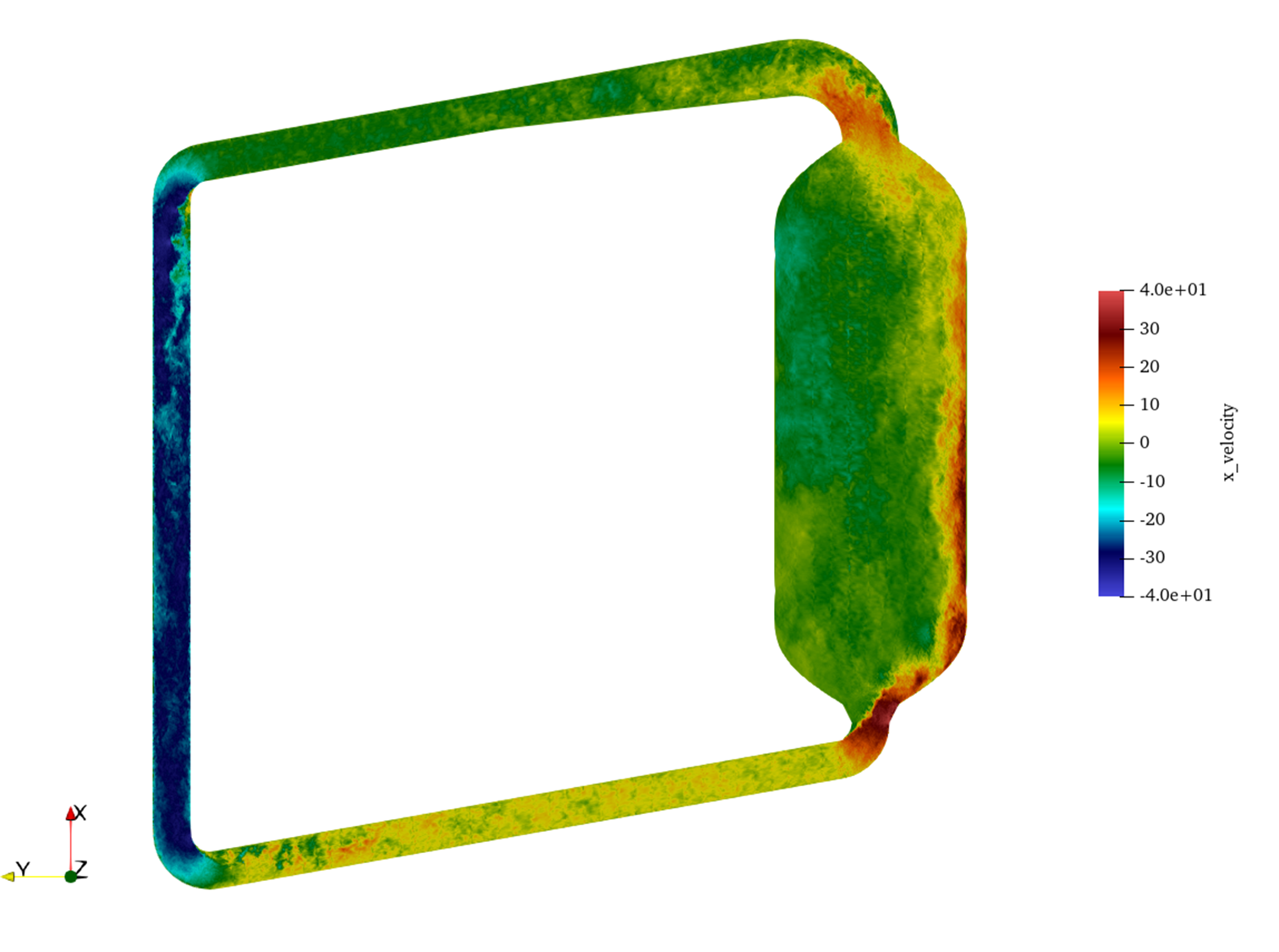
Figure 1: Instantaneous non-dimensional vertical velocity, , from the nekRS LES. The incoming jet is deflected by upstream curvature and produces strong local fluctuations.
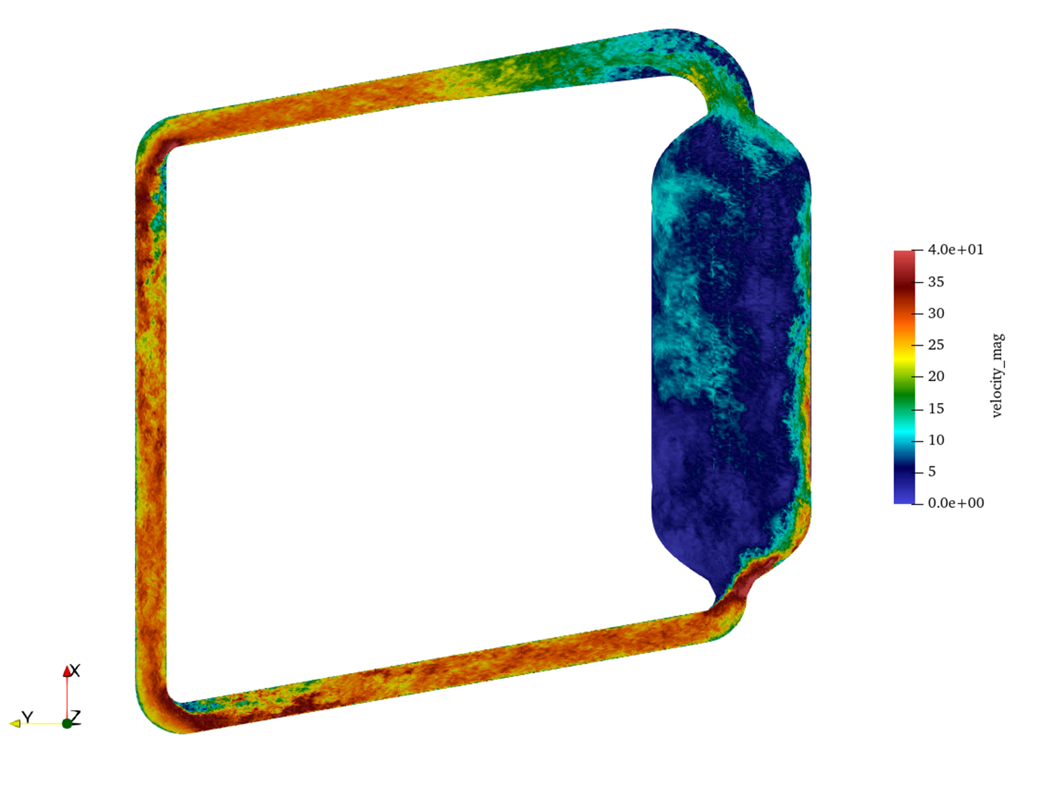
Figure 2: Instantaneous non-dimensional velocity magnitude, , showing energetic large-scale eddies in the open core cavity.
The strongest instantaneous velocities occur along the impingement side of the vessel, where the inlet momentum enters the larger core volume. This behavior has potential implications for local wall heat transfer, thermal striping, and structural vibration. It also demonstrates why a high-fidelity reference solution is valuable: a steady or overly diffusive turbulence model may smooth out the coherent jet path that governs loop-scale mixing.
Time-averaged flow structure
The time-averaged LES field reveals persistent macroscopic flow asymmetry. A high-velocity stream remains concentrated near the outer wall and a broad, low-velocity recirculating region occupies the opposite side of the core. The mean vertical velocity further indicates a complex three-dimensional recirculation pattern, including downward flow in the bulk region that competes with the wall-bounded inlet-to-outlet pathway.
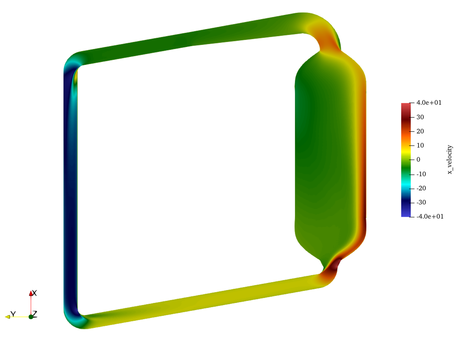
Figure 3: Time-averaged non-dimensional vertical velocity, , showing the persistent asymmetric circulation pattern.
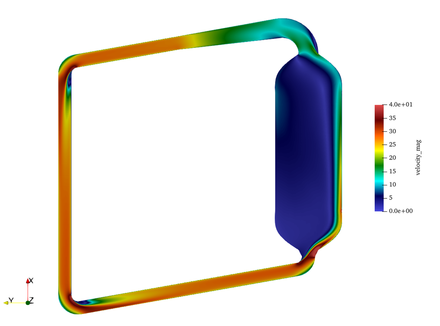
Figure 4: Time-averaged non-dimensional velocity magnitude, , highlighting the high-speed wall stream and lower-speed recirculation zones.
Three features are especially important for reactor analysis:
Flow short-circuiting: A substantial fraction of the fuel salt follows a fast wall-adjacent route from inlet to outlet. This path can reduce the effective core residence time for part of the fluid inventory and alter delayed neutron precursor transport.
Stagnation and dead zones: The side of the core opposite the inlet jet contains large regions of low mean velocity. In a coupled thermal calculation, such zones may be susceptible to heat accumulation because local advective removal is weak.
Three-dimensional recirculation: The combination of strong inlet curvature, expansion into an open vessel, and outlet suction generates a mean flow that cannot be adequately represented by a one-dimensional loop model or by an axisymmetric approximation.
Implications for Lower-Fidelity Model Calibration
The LES data provide a reference for calibrating RANS and coarse-mesh system models used in longer reactor transients. In particular, this high-fidelity model can support:
tuning of turbulent viscosity or turbulent kinetic energy limiters in stagnation and reattachment regions;
selection of mixing-length scales that preserve the observed large coherent structures rather than overdamping them;
assessment of wall-function behavior in regions of jet impingement, curvature-driven separation, and recirculation;
residence-time-distribution estimates for delayed neutron precursor transport in liquid-fueled MSR multiphysics simulations;
evaluation of whether porous-resistance or momentum-source surrogates in lower-fidelity tools reproduce the LES mean flow split and short-circuiting path.
Running the Case
A typical nekRS workflow is to run a lower-cost transient at a lower polynomial order to establish a turbulent state, and then restart at the production polynomial order () for time averaging. The simulation employs second-order time stepping (tombo2) by default. From the msr/lotus/les directory, launch the simulation (for example, with 4 MPI ranks using nrsmpi):
nrsmpi mcre 4
To restart the calculation at a higher polynomial order (e.g., transitioning from to for production averaging), update mcre.par under [GENERAL] by changing polynomialOrder and specifying the restart file with startFrom:
[GENERAL]
polynomialOrder = 7
startFrom = mcre0.f05000
No manual recompilation or preprocessing is needed after modifying mcre.par. When launched, nekRS automatically handles solution field interpolation between the different polynomial orders and continues the simulation using the standard run command:
nrsmpi mcre 4
For CPU-only testing or debugging, backend options can be specified as needed (e.g., --backend CPU or --backend CUDA). For production calculations, also ensure viscosity, numSteps, and checkpoint cadence in mcre.par match the target Reynolds number and averaging window.
References
- Paul Fischer, Stefan Kerkemeier, Misun Min, Yu-Hsiang Lan, Malachi Phillips, Thilina Rathnayake, Elia Merzari, Ananias Tomboulides, Ali Karakus, Noel Chalmers, and Tim Warburton.
NekRS, a GPU-accelerated spectral element Navier–Stokes solver.
Parallel Computing, 114:102982, 2022.[Export]
- Mauricio Tano, Ramiro Freile, Rodrigo de Oliveira, Samuel Walker, and Abdalla Abou-Jaoude.
Coupled steady-state precursor distribution, and transients studies for open-core flow mcfrs.
Technical Report INL/RPT-23-73982, Idaho National Laboratory, 2023.[Export]
- Dan Walter, Tommy Cisneros, Kent Wardle, Josh Walter, and Sean Findlay.
Mcre design description in support of external model development.
Technical Report MCRE-ENG-PRSNT-0029, TerraPower, 2022.[Export]