SAM System Model for the Molten Salt Separate Effects Loop (SEL)
Contact: Thanh Hua, thua.at.anl.gov; Jun Fang, fangj.at.anl.gov
Model link: SEL SAM System Model
Model Overview
The SEL SAM model is a system-level representation of the Molten Salt Separate Effects Loop (SEL). The working fluid is a molten salt mixture of MgCl2-NaCl. The model simulates the primary loop with forced convection (salt mass flow rate of 1 kg/s) in an electrically heated 1-pin test section configuration (11 kW heating power).
In addition to the primary loop, the model includes a secondary loop where pressurized air cools the primary heat exchanger (PHX) and is subsequently cooled by a water-based secondary heat exchanger (SHX) before being safely vented. This is in accordance with building safety requirements which mandate the air to be reduced in temperature (< 60°C) before venting to the environment.
The SAM model is designed to simulate both steady-state forced flow conditions and transient natural circulation scenarios, such as a loss of flow transient induced by a pump coast-down. The model is currently focused on a single-pin configuration but is structured to easily expand to 7-pin and conjugate heat transfer configurations in the future.
Input File Description
The model has two main input files:
OnepinSS.i: Simulates the steady-state operating conditions with forced flow.OnepinNC.i: Simulates a loss-of-flow transient (pump trip) and the resulting natural circulation.
The SAM input file adopts a block-structured syntax, and each block contains the detailed settings of specific SAM components. In this section, we will go through the important blocks in the input file and explain the key model specifications.
GlobalParams
This block contains the global parameters that are applied to all SAM components, such as the initial pressure (1.e5 Pa), initial velocity (2.0 m/s), and global initial temperature (773.15 K). This section also specifies variable scaling factors (scaling_factor_var = '1 1e-2 1e-5'), which is a crucial numerical setup in SAM (based on MOOSE's PJFNK solver). The simulation solves equations for mass, momentum and energy conservation that have drastically different magnitudes, scaling them improves matrix preconditioning and solver convergence.
[GlobalParams]
  global_init_P = 1.e5 # Global initial fluid pressure
  global_init_V = 2.0 # Global initial fluid velocity
  global_init_T = 773.15 # Global initial temperature for fluid and solid
  scaling_factor_var = '1 1e-2 1e-5'
[]
EOS (Equations of State)
This block specifies the material equations of state for the three working fluids in the system. The primary loop uses PTFunctionsEOS to define the temperature-dependent thermophysical properties of the molten salt (MgCl2-NaCl) via piece-wise linear interpolations (PiecewiseLinear functions defined in the Functions block). The secondary and tertiary loops use AirEquationOfState for pressurized air and PTConstantEOS for the cooling water, respectively.
The thermophysical properties for the molten salt were obtained via private communication with an ARPA-E project industry partner, as the primary source contains proprietary information.
[EOS]
  [salt_eos]
    type = PTFunctionsEOS
    rho = rho_coolant
    cp = 971.3 # MgCl2_NaCl
    mu = mu_coolant
    k = k_coolant
    T_min = 500
    T_max = 1500
  []
  [air_eos]
    type = AirEquationOfState
    p_0 = 3.4e5
  []
  [water_eos]
    type = PTConstantEOS
    rho_0 = 996.5
    p_0 = 1.0e5
    T_0 = 300.
    beta = 2.57e-4
    cp = 4182
    h_0 = 1.2546e6
    mu = 8.55e-4
    k = 0.613
  []
[]
Components
This is the main block in the input file. It provides the specifications for all physical components that make up the loop, converting the 3D facility geometry into an equivalent 1D system network using components such as the test section, heat exchangers, pumps, and connecting pipes.
The test section is modeled as a PBCoreChannel incorporating the electrically heated heater pin. Key parameters such as hydraulic diameter (Dh = 0.015494) and flow area are carefully specified to represent the annular flow path between the single heater pin and the surrounding pipe wall. Heat transfer correlations are tuned (SC_HTC = 1.3) to account for local flow phenomena:
[Components]
  [CH1]
    # Test section
    type = PBCoreChannel
    eos = salt_eos
    orientation = '0 0 1'
    position = '0 1.25 0.1'
    A = 0.000806
    Dh = 0.015494
    length = 0.5
    n_elems = 25

    HT_surface_area_density = 98.913
    HTC_geometry_type = Pipe
    dim_hs = 2
    name_of_hs = 'heater'
    Ts_init = 773.15
    n_heatstruct = 1
    fuel_type = cylinder
    width_of_hs = '0.0127' # radius of heater pin
    elem_number_of_hs = '5'
    material_hs = 'ss-mat'
    lam_factor = 1.4
    turb_factor = 1.1
    SC_HTC = 1.3 # enhance HTC by 30%
    power_fraction = 1.0 # Assign all power to the single heat structure
  []
[]
The primary (IHX) and secondary (SHX) heat exchangers are modeled using the PBHeatExchanger component, which simulates 1D counter-current heat exchange across a shared wall. The IHX couples the primary salt loop to the pressurized air loop, while the SHX couples the air loop to the final water cooling sink, allowing the air to be safely discharged to the environment below 60°C:
[Components]
  [IHX]
    type = PBHeatExchanger
    eos = salt_eos
    eos_secondary = air_eos
    orientation = '0.996180782 -0.087314654 0'
    position = '0 0.9 0.8'
    length = 5.7264
    n_elems = 100

    A = 3.5244E-04
    Dh = 2.1184E-02
    HT_surface_area_density = 226.4093
    A_secondary = 1.2891E-04
    Dh_secondary = 3.0480E-03
    HT_surface_area_density_secondary = 619.0264

    heat_transfer_area_error_tolerance = 0.002
    f = 0.02
    initial_V_secondary = -80
    Hw = 350
    Hw_secondary = 1500
    wall_thickness = 2.1082E-03
    Twall_init = 773.15
    dim_wall = 2
    n_wall_elems = 1
    material_wall = ss-mat
  []
[]
The molten salt pump (Pump_p) uses a PBPump component to drive forced convection. Its pressure head is defined via a time-dependent function (pump_head) that is central to both the steady-state and transient simulations. To reach the steady-state initial condition, the pump head is held at a constant value from a pseudo-transient start time of -20,000 s up to 0 s to establish a steady 1 kg/s salt mass flow rate. For transient loss of flow simulations, a pump trip is initiated at time > 0, where the pump head function coasts down towards zero.
[Components]
  [Pump_p]
    type = PBPump
    eos = salt_eos
    inputs = 'Pipe5(out)'
    outputs = 'Pipe6(in)'
    K = '0.15 0.1'
    Area = 0.001313436
    initial_P = 1.e5
    #    Head      = 1.25e4 #2.25e3
    Head = pump_head
  []
[]
Postprocessors
The Postprocessors block is used to extract and monitor macroscopic quantities of interest during the simulation, such as mass flow rates, average temperatures, and total heat transfer. These values are printed to the console and saved to a CSV file to easily verify steady-state energy balances and track transient behaviors.
[Postprocessors]
  [CH1_flow]
    # Output mass flow rate at inlet of CH1
    type = ComponentBoundaryFlow
    input = CH1(in)
  []

  [air_flow]
    # Output mass flow rate at secondary inlet of IHX
    type = ComponentBoundaryFlow
    input = IHX(secondary_in)
  []

  [water_flow]
    # Output mass flow rate at secondary inlet of SHX
    type = ComponentBoundaryFlow
    input = SHX(secondary_in)
  []

  [CH1_velocity]
    # Output velocity at inlet of CH1
    type = ComponentBoundaryVariableValue
    variable = velocity
    input = CH1(in)
  []

  [CH1_Tin]
    # Temperature at inlet of CH1
    type = ComponentBoundaryVariableValue
    variable = temperature
    input = CH1(in)
  []

  [CH1_Tout]
    # Temperature at outlet of CH1
    type = ComponentBoundaryVariableValue
    variable = temperature
    input = CH1(out)
  []

  [IHX_Tin_p]
    # Temperature at IHX inlet
    type = ComponentBoundaryVariableValue
    variable = temperature
    input = IHX(primary_in)
  []

  [IHX_Tout_p]
    # Temperature at IHX outlet
    type = ComponentBoundaryVariableValue
    variable = temperature
    input = IHX(primary_out)
  []

  [IHX_Tin_s]
    # Temperature at IHX secondary inlet
    type = ComponentBoundaryVariableValue
    variable = temperature
    input = IHX(secondary_in)
  []

  [IHX_Tout_s]
    # Temperature at IHX secondary outlet
    type = ComponentBoundaryVariableValue
    variable = temperature
    input = IHX(secondary_out)
  []

  [SHX_Tin_p]
    # Temperature at SHX inlet
    type = ComponentBoundaryVariableValue
    variable = temperature
    input = SHX(primary_in)
  []

  [SHX_Tout_p]
    # Temperature at SHX outlet
    type = ComponentBoundaryVariableValue
    variable = temperature
    input = SHX(primary_out)
  []

  [SHX_Tin_s]
    # Temperature at SHX secondary inlet
    type = ComponentBoundaryVariableValue
    variable = temperature
    input = SHX(secondary_in)
  []

  [SHX_Tout_s]
    # Temperature at SHX secondary outlet
    type = ComponentBoundaryVariableValue
    variable = temperature
    input = SHX(secondary_out)
  []

  [HX_E]
    type = ComponentBoundaryEnergyBalance
    eos = salt_eos
    input = 'IHX(primary_out) IHX(primary_in)'
  []

  [./HX_SE]
    type = ComponentBoundaryEnergyBalance
    eos = air_eos
    input = 'IHX(secondary_out) IHX(secondary_in)'
  [../]

  [SHX_E]
    type = ComponentBoundaryEnergyBalance
    eos = air_eos
    input = 'SHX(primary_out) SHX(primary_in)'
  []

  [./SHX_SE]
    type = ComponentBoundaryEnergyBalance
    eos = water_eos
    input = 'SHX(secondary_out) SHX(secondary_in)'
  [../]
[]
Executioner
This block orchestrates the overall calculation process flow. It sets the solver type (e.g., Transient), start time, end time, and time-stepping scheme. It also configures the PETSc solver options (such as using the lu preconditioner with petsc_options_iname='-pc_type' and petsc_options_value = 'lu') to ensure that the solve for the non-linear fluid flow and conjugate heat transfer equations converge efficiently.
[Executioner]
  type = Transient
  start_time = -20000
  end_time = 0
  dt = 1.00
  dtmin = 1e-4
  dtmax = 200.0

  [TimeStepper]
    type = IterationAdaptiveDT
    dt = 0.1
    growth_factor = 1.5
    optimal_iterations = 10
  []

  petsc_options_iname = '-ksp_gmres_restart -pc_type'
  petsc_options_value = '300 lu'
  nl_rel_tol = 1e-4
  nl_abs_tol = 1e-4
  nl_max_its = 30

  l_tol = 1e-4 # Relative linear tolerance for each Krylov solve
  l_max_its = 100 # Number of linear iterations for each Krylov solve

  [Quadrature]
    type = TRAP
    order = FIRST
  []
[]
Results
Steady State Operating Conditions
For a base case, salt flow rate 1 kg/s, and heater power of 11 kW:
11.3 K coolant temperature rise
Peak pin centerline temperature 1135 K, pin surface temperature 1008 K
Air temperature rises to 780 K in PHX, cools down to 312.3 K in SHX for discharge to the environment.
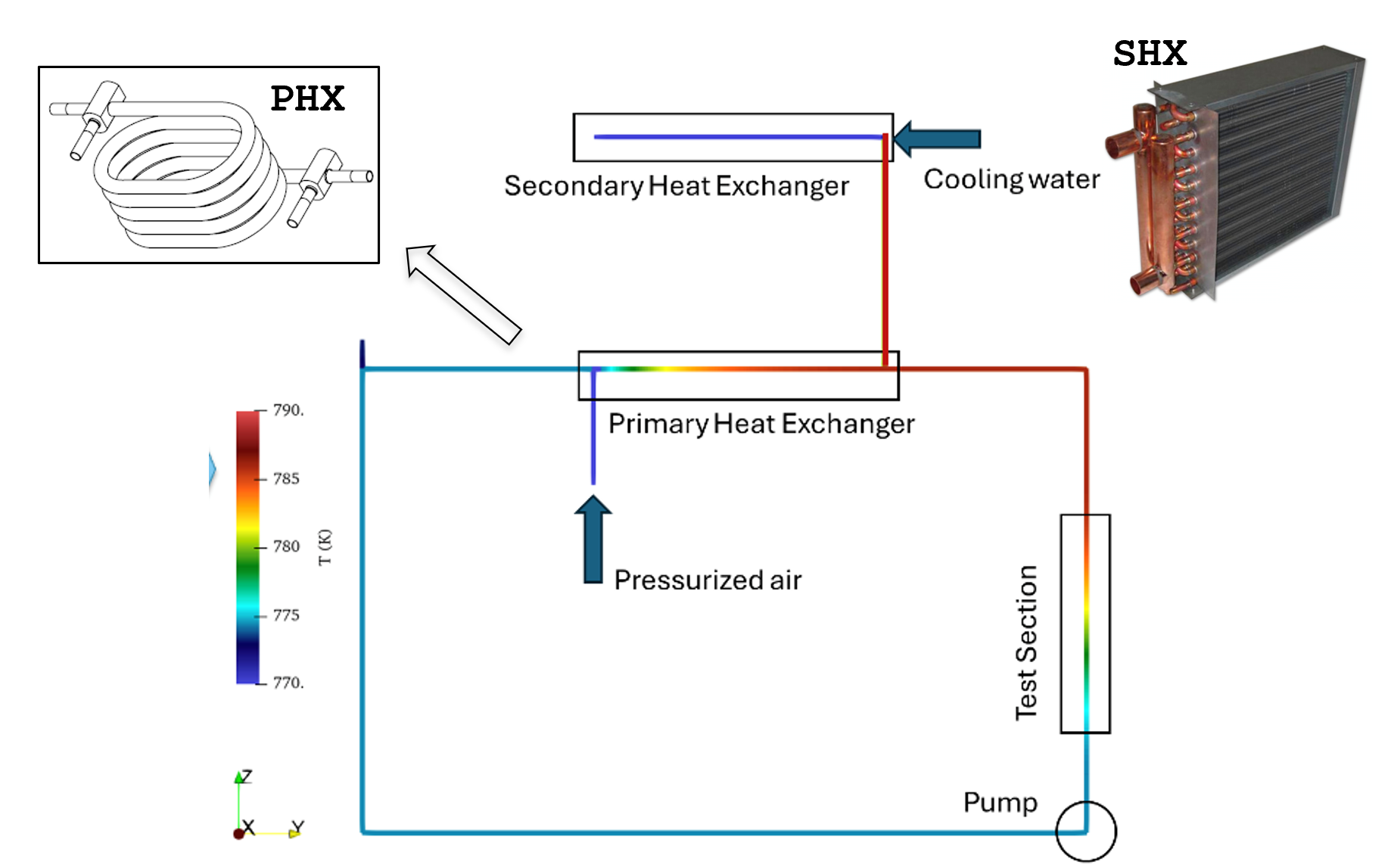
Figure 1: Steady State Loop Temperature
Table 1: Steady State Operating Conditions
| Component | Fluid | Inlet Temperature (K) | Outlet Temperature (K) | Mass flow rate (kg/s) |
|---|---|---|---|---|
| PHX | Salt | 772.5 | 783.8 | 1.0 |
| PHX | Air | 300.0 | 781.3 | 0.022 |
| SHX | Air | 778.2 | 312.3 | 0.022 |
| SHX | Water | 300.0 | 319.8 | 0.13 |
Natural Circulation in Pump Trip Transient
To simulate a loss-of-flow scenario, a pump trip is initiated at . The pump head is programmed to coast down, eventually reaching zero at seconds.
Flow Transition: As the forced flow decays, the flow rate drops from the initial 1.0 kg/s but does not go to zero. Instead, a stable natural circulation flow of approximately 0.12 kg/s is successfully established in the loop, driven by the buoyancy difference between the hot salt in the heater test section and the cooler salt in the heat exchangers.
Test Section Temperatures: Due to the significantly reduced mass flow rate under constant 11 kW heating, the temperature rise across the test section () increases dramatically. The salt inlet temperature gradually drops to ~700 K as cooler salt returns from the PHX. Meanwhile, the outlet temperature experiences a transient peak near 825 K before settling around 795 K. This results in a steady-state natural circulation of approximately 95 K, up from the initial 11.3 K in forced flow.
Heat Exchanger Performance: Both the primary (PHX) and secondary (SHX) heat exchangers continue to operate effectively throughout the transient. In the PHX, the air outlet temperature smoothly tracks the transient peak of the incoming hot salt. Crucially, the SHX continues to successfully dump this heat into the water cooling sink, maintaining an extremely stable air discharge temperature of ~312–314 K (well below the 60°C / 333 K facility safety requirement).
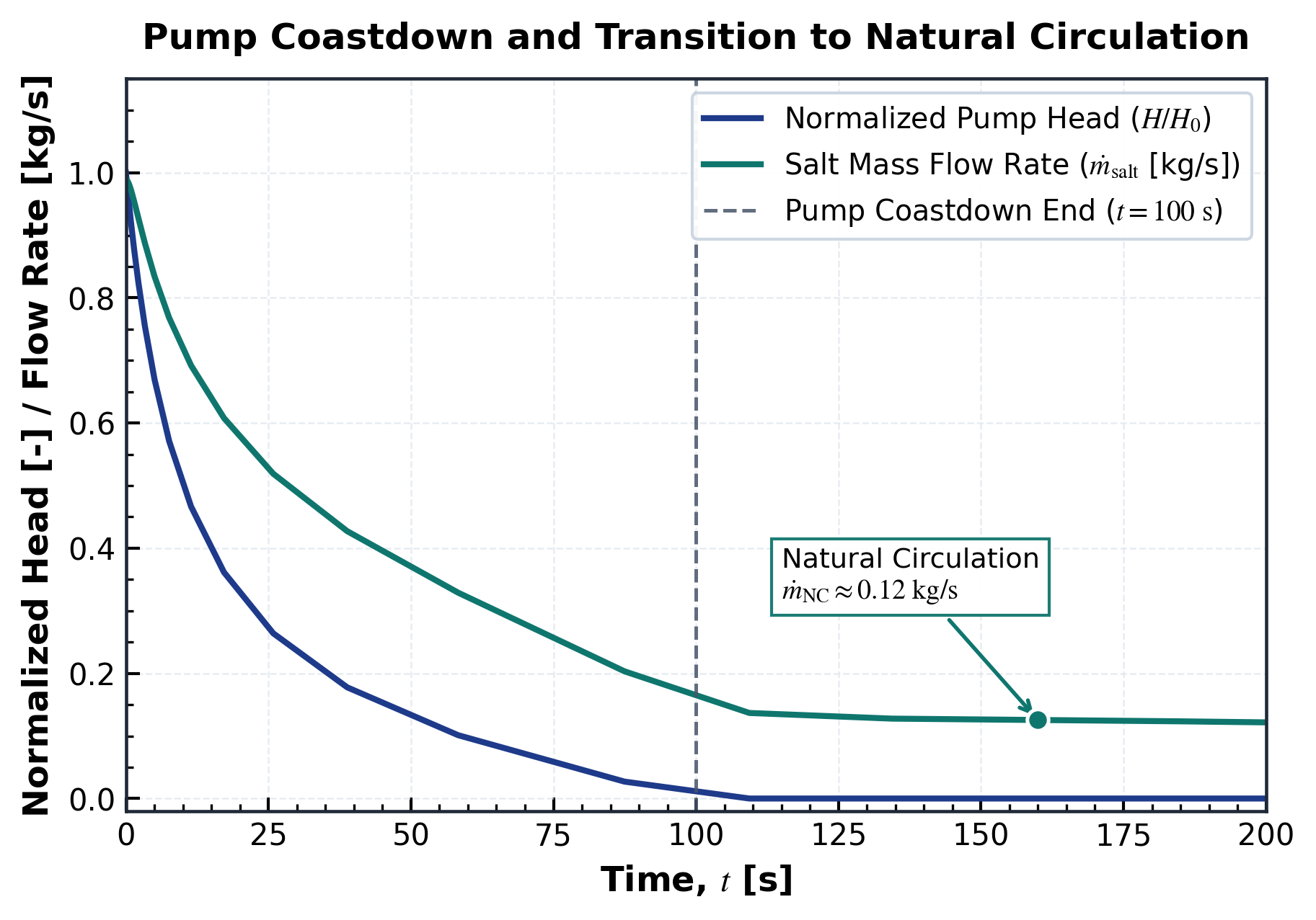
Figure 2: Normalized Pump Head and Flow Rate During the Transient
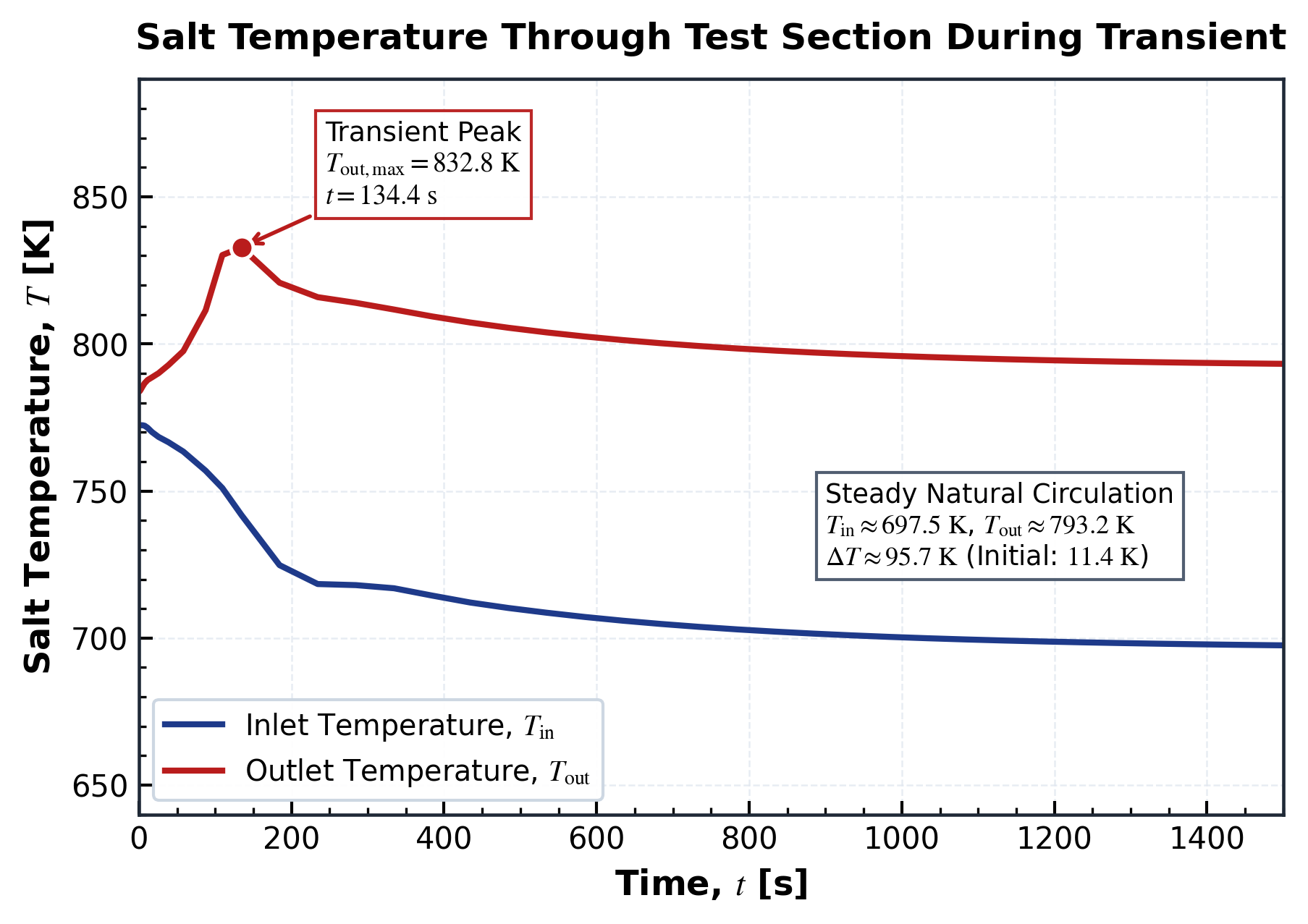
Figure 3: Transient Salt Temperatures at Test Section Inlet and Outlet
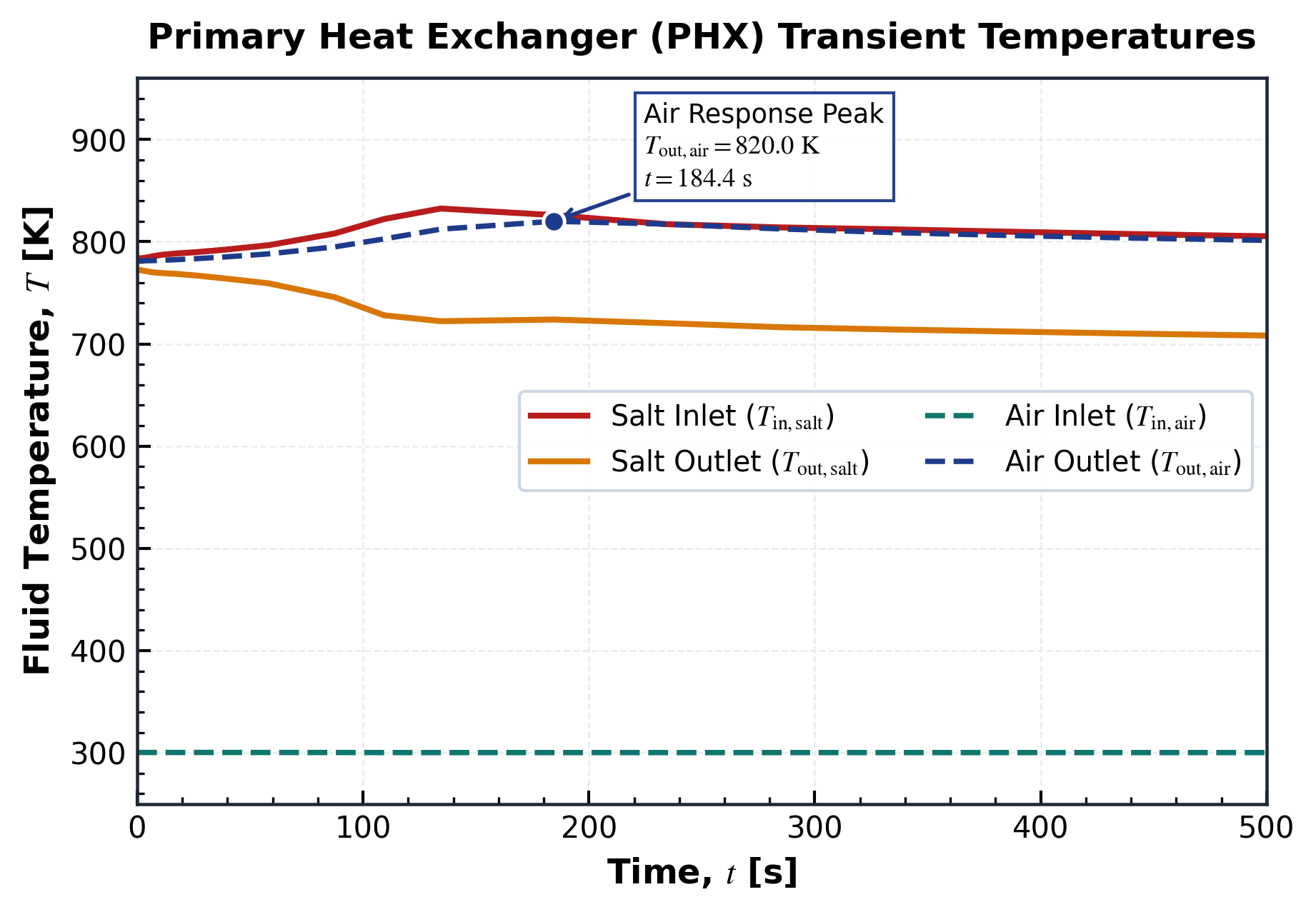
Figure 4: Transient Fluid Temperatures on Both Sides of PHX
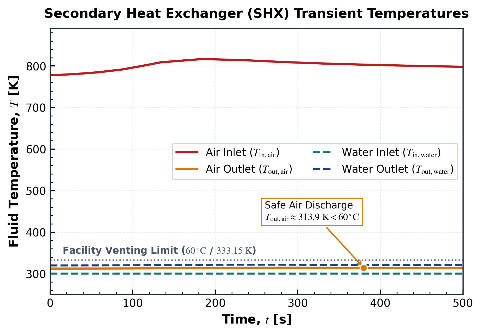
Figure 5: Transient Fluid Temperatures on Both Sides of SHX
Run Command
Both the steady-state and transient models are lightweight and can be run efficiently on a local workstation or laptop. Note that the transient input model relies on the final checkpoint file from the steady-state case to set its initial condition. Therefore, the steady-state model must be run first.
Below is a simple example of how to run the models sequentially:
# Run the steady-state case first to generate the checkpoint file
/path/to/sam-opt -i OnepinSS.i

# Run the transient case
/path/to/sam-opt -i OnepinNC.i
(msr/sel/OnepinSS.i)
# ==============================================================================
# Model: Molten Salt Separate Effects Loop (SEL)
# Application: SAM (System Analysis Module)
# Simulation: Steady-state forced flow operating conditions (1 kg/s, 11 kW)
# ------------------------------------------------------------------------------
# Author(s): Thanh Hua ([email protected]), Jun Fang ([email protected])
# Institution: Argonne National Laboratory (ANL)
# Sponsor: ARPA-E
# If using or referring to this model, please cite as explained on
# https://mooseframework.inl.gov/virtual_test_bed/citing.html
# ==============================================================================
[GlobalParams]
global_init_P = 1.e5 # Global initial fluid pressure
global_init_V = 2.0 # Global initial fluid velocity
global_init_T = 773.15 # Global initial temperature for fluid and solid
scaling_factor_var = '1 1e-2 1e-5'
[]
[EOS]
[salt_eos]
type = PTFunctionsEOS
rho = rho_coolant
cp = 971.3 # MgCl2_NaCl
mu = mu_coolant
k = k_coolant
T_min = 500
T_max = 1500
[]
[air_eos]
type = AirEquationOfState
p_0 = 3.4e5
[]
[water_eos]
type = PTConstantEOS
rho_0 = 996.5
p_0 = 1.0e5
T_0 = 300.
beta = 2.57e-4
cp = 4182
h_0 = 1.2546e6
mu = 8.55e-4
k = 0.613
[]
[]
[Functions]
[rho_coolant] #2125.3 - 0.47419T (T in K) MgCl2-NaCl
type = PiecewiseLinear
x = '500 600 700 800 900 1000 1100 1200 1300 1400 1500'
y = '1888.205 1840.786 1793.367 1745.948 1698.529 1651.11 1603.691 1556.272 1508.853 1461.434 1414.015'
[]
[mu_coolant] #53853.2*T^(-2.55901) (T in K)
type = PiecewiseLinear
x = '500 600 700 800 900 1000 1100 1200 1300 1400 1500'
y = '0.006676061 0.00418692 0.002822131 0.002005281 0.001483458 0.001132874 0.000887682 0.000710487 0.000578894 0.000478893 0.000401386'
[]
[k_coolant] #0.047+0.0005 (T in K)
type = PiecewiseLinear
x = '500 600 700 800 900 1000 1100 1200 1300 1400 1500'
y = '0.297 0.347 0.397 0.447 0.497 0.547 0.597 0.647 0.697 0.747 0.797'
[]
[pump_head]
type = PiecewiseLinear
x = '-20000 0 0.5 1 1.5 2 2.5 3 3.5 4 4.5
5 5.5 6 6.5 7 7.5 8 8.5 9 9.5
10 12 14 16 18 20 22 24 26 28
30 32 34 36 38 40 42 44 46 48
50 55 60 65 70 75 80 85 90 95 100 1.00E+05'
y = '1 1 0.953667299 0.91134767 0.872537608 0.836814455 0.803820794 0.773252333 0.744848383 0.718384322 0.693665564
0.670522702 0.648807559 0.62838997 0.609155121 0.591001349 0.573838317 0.557585476 0.542170772 0.527529561 0.513603673
0.500340627 0.4530308 0.413216875 0.37919713 0.349748106 0.323967566 0.301175519 0.280849718 0.262582382 0.246050431
0.230994538 0.217204114 0.204506338 0.19275802 0.181839483 0.171649895 0.162103673 0.153127675 0.14465899 0.136643183
0.129032883 0.111521369 0.095773409 0.0813972 0.068092284 0.055621852 0.043794013 0.032448693 0.021448129 0.010669661 0 0'
scale_factor = 1.3e4 # required pump head
[]
[]
[MaterialProperties]
[ss-mat]
type = SolidMaterialProps
k = 20
Cp = 638
rho = 7.7e3
[]
[]
[Components]
[reactor]
type = ReactorPower
initial_power = 11000
[]
[CH1] # Test section
type = PBCoreChannel
eos = salt_eos
orientation = '0 0 1'
position = '0 1.25 0.1'
A = 0.000806
Dh = 0.015494
length = 0.5
n_elems = 25
HT_surface_area_density = 98.913
HTC_geometry_type = Pipe
dim_hs = 2
name_of_hs = 'heater'
Ts_init = 773.15
n_heatstruct = 1
fuel_type = cylinder
width_of_hs = '0.0127' # radius of heater pin
elem_number_of_hs = '5'
material_hs = 'ss-mat'
lam_factor = 1.4
turb_factor = 1.1
SC_HTC = 1.3 # enhance HTC by 30%
power_fraction = 1.0 # Assign all power to the single heat structure
[]
[Pipe1] # (to HX)
type = PBOneDFluidComponent
orientation = '0 0 1'
position = '0 1.25 0.6'
length = 0.2
A = 0.001313436
Dh = 0.040894
n_elems = 4
eos = salt_eos
[]
[Pipe2] # (to HX)
type = PBOneDFluidComponent
orientation = '0 -1 0'
position = '0 1.25 0.8'
length = 0.35
A = 0.001313436
Dh = 0.040894
n_elems = 7
eos = salt_eos
[]
[IHX]
type = PBHeatExchanger
eos = salt_eos
eos_secondary = air_eos
orientation = '0.996180782 -0.087314654 0'
position = '0 0.9 0.8'
length = 5.7264
n_elems = 100
A = 3.5244E-04
Dh = 2.1184E-02
HT_surface_area_density = 226.4093
A_secondary = 1.2891E-04
Dh_secondary = 3.0480E-03
HT_surface_area_density_secondary = 619.0264
heat_transfer_area_error_tolerance= 0.002
f = 0.02
initial_V_secondary = -80
Hw = 350
Hw_secondary = 1500
wall_thickness = 2.1082E-03
Twall_init = 773.15
dim_wall = 2
n_wall_elems = 1
material_wall = ss-mat
[]
[inlet_air]
type = PBTDJ
input = 'Pipe8(in)'
eos = air_eos
v_bc = 24. #34.5
T_bc = 300 #394.25
[]
[Pipe8] # (air inflow to secondary side of IHX)
type = PBOneDFluidComponent
orientation = '0 0 1'
position = '0 0.4 0.6'
length = 0.2
A = 1.2891E-04
Dh = 3.0480E-03
n_elems = 4
eos = air_eos
[]
[Branch8]
type = PBSingleJunction
inputs = 'Pipe8(out)'
outputs = 'IHX(secondary_in)'
eos = air_eos
[]
[Pipe9] # (air outflow from secondary side of IHX)
type = PBOneDFluidComponent
orientation = '0 0 1'
position = '0 0.9 0.8'
length = 0.4
A = 1.2891E-04
Dh = 3.0480E-03
n_elems = 8
eos = air_eos
[]
[Branch9]
type = PBSingleJunction
inputs = 'IHX(secondary_out)'
outputs = 'Pipe9(in)'
eos = air_eos
[]
[outlet_air]
type = PBTDV
input = 'SHX(primary_out)'
eos = air_eos
p_bc = 3.4e5
[]
[Branch10]
type = PBBranch
inputs = 'Pipe9(out)'
outputs = 'SHX(primary_in)'
K = '0.0 0.0'
Area = 0.013
eos = air_eos
[]
[SHX]
type = PBHeatExchanger
eos = air_eos
eos_secondary = water_eos
orientation = '0 -1 0'
position = '0 0.9 1.2'
length = 0.5
n_elems = 25
A = 0.013
Dh = 0.01
HT_surface_area_density = 1e2
A_secondary = 0.0013
Dh_secondary = 0.01
HT_surface_area_density_secondary = 1e3
heat_transfer_area_error_tolerance= 0.002
f = 0.02
initial_V_secondary = -10
Hw = 400
Hw_secondary = 200
wall_thickness = 0.0015
Twall_init = 773.15
dim_wall = 2
n_wall_elems = 1
material_wall = ss-mat
[]
[inlet_water]
type = PBTDJ
input = 'SHX(secondary_in)'
eos = water_eos
v_bc = -0.1
T_bc = 300
[]
[outlet_water]
type = PBTDV
input = 'SHX(secondary_out)'
eos = water_eos
p_bc = 1.0e5
[]
[Pipe3] # (from HX)
type = PBOneDFluidComponent
orientation = '0 -1 0'
position = '0 0.4 0.8'
length = 0.4
A = 0.001313436
Dh = 0.040894
n_elems = 8
eos = salt_eos
[]
[Pipe4] # (downcomer)
type = PBOneDFluidComponent
orientation = '0 0 -1'
position = '0 0 0.8'
length = 0.8
A = 0.001313436
Dh = 0.040894
n_elems = 16
eos = salt_eos
[]
[Pipe5] # (to pump)
type = PBOneDFluidComponent
orientation = '0 1 0'
position = '0 0 0'
length = 1.25
A = 0.001313436
Dh = 0.040894
n_elems = 25
eos = salt_eos
[]
[Pipe6] # (to CH1)
type = PBOneDFluidComponent
orientation = '0 0 1'
position = '0 1.25 0'
length = 0.1
A = 0.001313436
Dh = 0.040894
n_elems = 2
eos = salt_eos
[]
[Pipe7] # (ref)
type = PBOneDFluidComponent
orientation = '0 0 1'
position = '0 0 0.8'
length = 0.05
A = 0.001313436
Dh = 0.040894
n_elems = 2
eos = salt_eos
[]
[Branch1]
type = PBSingleJunction
inputs = 'CH1(out)'
outputs = 'Pipe1(in)'
eos = salt_eos
[]
[Branch2]
type = PBSingleJunction
inputs = 'Pipe1(out)'
outputs = 'Pipe2(in)'
eos = salt_eos
[]
[Branch3]
type = PBBranch
inputs = 'Pipe2(out)'
outputs = 'IHX(primary_in)'
K = '0.0 0.0'
Area = 0.001313436
eos = salt_eos
[]
[Branch4]
type = PBBranch
inputs = 'IHX(primary_out)'
outputs = 'Pipe3(in)'
K = '0.0 0.0'
Area = 0.001313436
eos = salt_eos
[]
[Branch5]
type = PBBranch
inputs = 'Pipe3(out)'
outputs = 'Pipe4(in) Pipe7(in)'
K = '0.0 0.0 10.0'
Area = 0.001313436
initial_P = 1e5
eos = salt_eos
[]
[Branch6]
type = PBSingleJunction
inputs = 'Pipe4(out)'
outputs = 'Pipe5(in)'
eos = salt_eos
[]
[Pump_p]
type = PBPump
eos = salt_eos
inputs = 'Pipe5(out)'
outputs = 'Pipe6(in)'
K = '0.15 0.1'
Area = 0.001313436
initial_P = 1.e5
# Head = 1.25e4 #2.25e3
Head = pump_head
[]
[Branch7]
type = PBSingleJunction
inputs = 'Pipe6(out)'
outputs = 'CH1(in)'
eos = salt_eos
[]
[p_out]
type = PBTDV
input = 'Pipe7(out)'
eos = salt_eos
p_bc = 1e5
T_bc = 773.15
[]
[]
[VectorPostprocessors]
[CH1_temp]
type = NodalValueSampler
variable = temperature
block = 'CH1:pipe'
sort_by = z
outputs = 'CH1_temp'
[]
[CH1pin_temp]
type = NodalValueSampler
variable = T_solid
block = 'CH1:solid:heater'
sort_by = z
outputs = 'CH1pin_temp'
[]
[]
[Postprocessors]
[CH1_flow] # Output mass flow rate at inlet of CH1
type = ComponentBoundaryFlow
input = CH1(in)
[]
[air_flow] # Output mass flow rate at secondary inlet of IHX
type = ComponentBoundaryFlow
input = IHX(secondary_in)
[]
[water_flow] # Output mass flow rate at secondary inlet of SHX
type = ComponentBoundaryFlow
input = SHX(secondary_in)
[]
[CH1_velocity] # Output velocity at inlet of CH1
type = ComponentBoundaryVariableValue
variable = velocity
input = CH1(in)
[]
[CH1_Tin] # Temperature at inlet of CH1
type = ComponentBoundaryVariableValue
variable = temperature
input = CH1(in)
[]
[CH1_Tout] # Temperature at outlet of CH1
type = ComponentBoundaryVariableValue
variable = temperature
input = CH1(out)
[]
[IHX_Tin_p] # Temperature at IHX inlet
type = ComponentBoundaryVariableValue
variable = temperature
input = IHX(primary_in)
[]
[IHX_Tout_p] # Temperature at IHX outlet
type = ComponentBoundaryVariableValue
variable = temperature
input = IHX(primary_out)
[]
[IHX_Tin_s] # Temperature at IHX secondary inlet
type = ComponentBoundaryVariableValue
variable = temperature
input = IHX(secondary_in)
[]
[IHX_Tout_s] # Temperature at IHX secondary outlet
type = ComponentBoundaryVariableValue
variable = temperature
input = IHX(secondary_out)
[]
[SHX_Tin_p] # Temperature at SHX inlet
type = ComponentBoundaryVariableValue
variable = temperature
input = SHX(primary_in)
[]
[SHX_Tout_p] # Temperature at SHX outlet
type = ComponentBoundaryVariableValue
variable = temperature
input = SHX(primary_out)
[]
[SHX_Tin_s] # Temperature at SHX secondary inlet
type = ComponentBoundaryVariableValue
variable = temperature
input = SHX(secondary_in)
[]
[SHX_Tout_s] # Temperature at SHX secondary outlet
type = ComponentBoundaryVariableValue
variable = temperature
input = SHX(secondary_out)
[]
[HX_E]
type = ComponentBoundaryEnergyBalance
eos = salt_eos
input = 'IHX(primary_out) IHX(primary_in)'
[]
[./HX_SE]
type = ComponentBoundaryEnergyBalance
eos = air_eos
input = 'IHX(secondary_out) IHX(secondary_in)'
[../]
[SHX_E]
type = ComponentBoundaryEnergyBalance
eos = air_eos
input = 'SHX(primary_out) SHX(primary_in)'
[]
[./SHX_SE]
type = ComponentBoundaryEnergyBalance
eos = water_eos
input = 'SHX(secondary_out) SHX(secondary_in)'
[../]
[]
[Preconditioning]
[SMP_PJFNK]
type = SMP
full = true
solve_type = 'PJFNK'
[]
[]
[Executioner]
type = Transient
start_time = -20000
end_time = 0
dt = 1.00
dtmin = 1e-4
dtmax = 200.0
[TimeStepper]
type = IterationAdaptiveDT
dt = 0.1
growth_factor = 1.5
optimal_iterations = 10
[]
petsc_options_iname = '-ksp_gmres_restart -pc_type'
petsc_options_value = '300 lu'
nl_rel_tol = 1e-4
nl_abs_tol = 1e-4
nl_max_its = 30
l_tol = 1e-4 # Relative linear tolerance for each Krylov solve
l_max_its = 100 # Number of linear iterations for each Krylov solve
[Quadrature]
type = TRAP
order = FIRST
[]
[]
[Outputs]
print_linear_residuals = false
perf_graph = true
checkpoint = true
[out_displaced]
type = Exodus
use_displaced = true
execute_on = 'initial timestep_end'
sequence = false
[]
[csv]
type = CSV
[]
[console]
type = Console
execute_scalars_on = 'none'
[]
[CH1_temp]
type = CSV
file_base = cool/CH1_temp
sync_times = '0.0'
sync_only = true
[]
[CH1pin_temp]
type = CSV
file_base = pin/CH1pin_temp
sync_times = '0.0'
sync_only = true
[]
[]