Micro Reactor Drum Rotation
Contact: Zachary Prince, zachary.prince.at.inl.gov, Yaqi Wang, yaqi.wang.at.inl.gov
Model link: Micro Reactor Drum Rotation Model
Reactor Description
This reactor model is based on the prototypical micro reactor presented in Terlizzi and Labouré (2023). The design is based on the Empire reactor (Matthews et al., 2021) with modifications made to ensure a negative overall temperature reactivity coefficient, necessary to simulate realistic transients. This 2 MWth core consists of 18 hexagonal assemblies arranged in two rings and surrounded by 12 control drums contained within a radial reflector. Each assembly is composed of 96 fuel pins, 60 moderator pins, and 61 heat pipes. Detailed dimensions and material composition can be found in Terlizzi and Labouré (2023).
This model has been simplified to a 2D geometry that leverages symmetry to reduce the domain to a 1/12th of the full core. Furthermore, the heat pipes are simulated using a convective boundary conditions, as opposed to using Sockeye to calculate the actual heat removal. Prince et al. (2023) presents the 3D version of this model.
The purpose of this exposition is to show how to perform a multiphysics transient simulation involving control drum rotation using Griffin. Initially, the drum is positioned halfway at 90 degrees. The drum is then rotated outward (inserting reactivity) at 20 degrees per second for two seconds, then rotated inward (removing reactivity) at 20 degrees per second for three seconds. Thus, the total transient duration is five seconds. Due to the symmetry imposed on the model, rotating this drum is equivalent to rotating all the drums in the core.
Model Description
Mesh
The following creates a mesh of the entire core:
Listing 1: Mesh blocks for full-core fine mesh.
[Mesh]
  [FUEL_pin]
    type = PolygonConcentricCircleMeshGenerator
    num_sides = 6 # must be six to use hex pattern
    num_sectors_per_side = '2 2 2 2 2 2'
    background_intervals = 1
    background_block_ids = '8'
    background_block_names = 'MONOLITH'
    polygon_size = 1.075
    polygon_size_style = 'apothem'
    ring_radii = '1.0'
    ring_intervals = '3'
    ring_block_ids = '1 2'
    ring_block_names = 'FUEL FUEL_QUAD'
    preserve_volumes = on
    quad_center_elements = false
  []

  [MOD_pin]
    type = PolygonConcentricCircleMeshGenerator
    num_sides = 6 # must be six to use hex pattern
    num_sectors_per_side = '2 2 2 2 2 2'
    background_intervals = 1
    background_block_ids = '8'
    background_block_names = 'MONOLITH'
    polygon_size = 1.075
    polygon_size_style = 'apothem'
    ring_radii = '0.975 1'
    ring_intervals = '3 1'
    ring_block_ids = '3 4 5'
    ring_block_names = 'MOD MOD_QUAD MGAP'
    preserve_volumes = on
    quad_center_elements = false
  []

  [HPIPE_pin]
    type = PolygonConcentricCircleMeshGenerator
    num_sides = 6 # must be six to use hex pattern
    num_sectors_per_side = '2 2 2 2 2 2'
    background_intervals = 1
    background_block_ids = '8'
    background_block_names = 'MONOLITH'
    polygon_size = 1.075
    polygon_size_style = 'apothem'
    ring_radii = '1.0'
    ring_intervals = '3'
    ring_block_ids = '6 7'
    ring_block_names = 'HPIPE HPIPE_QUAD'
    preserve_volumes = on
    quad_center_elements = false
  []

  [AIRHOLE_CELL]
    type = PolygonConcentricCircleMeshGenerator
    num_sides = 6 # must be six to use hex pattern
    num_sectors_per_side = '2 2 2 2 2 2'
    background_intervals = 3
    background_block_ids = '20 21'
    background_block_names = 'AIRHOLE AIRHOLE_QUAD'
    polygon_size = 1.075
    polygon_size_style = 'apothem'
    preserve_volumes = on
    quad_center_elements = false
  []

  [REFL_CELL]
    type = PolygonConcentricCircleMeshGenerator
    num_sides = 6 # must be six to use hex pattern
    num_sectors_per_side = '2 2 2 2 2 2'
    background_intervals = 2
    background_block_ids = '14 15'
    background_block_names = 'REFL REFL_QUAD'
    polygon_size = 1.075
    polygon_size_style = 'apothem'
    preserve_volumes = on
    quad_center_elements = false
  []

  [Assembly_1]
    type = PatternedHexMeshGenerator
    inputs = 'MOD_pin HPIPE_pin FUEL_pin'
    # Pattern ID  0        1        2
    background_intervals = 1
    background_block_id = '8'
    background_block_name = 'MONOLITH'
    duct_sizes = '16.0765'
    duct_sizes_style = 'apothem'
    duct_block_ids = '22'
    duct_block_names = 'AIR'
    duct_intervals = 1
    hexagon_size = '16.1765'
    pattern = '1 0 1 0 1 0 1 0 1;
              0 2 2 2 2 2 2 2 2 0;
             1 2 1 0 1 0 1 0 1 2 1;
            0 2 0 2 2 2 2 2 2 0 2 0;
           1 2 1 2 1 0 1 0 1 2 1 2 1;
          0 2 0 2 0 2 2 2 2 0 2 0 2 0;
         1 2 1 2 1 2 1 0 1 2 1 2 1 2 1;
        0 2 0 2 0 2 0 2 2 0 2 0 2 0 2 0;
       1 2 1 2 1 2 1 2 1 2 1 2 1 2 1 2 1;
        0 2 0 2 0 2 0 2 2 0 2 0 2 0 2 0;
         1 2 1 2 1 2 1 0 1 2 1 2 1 2 1;
          0 2 0 2 0 2 2 2 2 0 2 0 2 0;
           1 2 1 2 1 0 1 0 1 2 1 2 1;
            0 2 0 2 2 2 2 2 2 0 2 0;
             1 2 1 0 1 0 1 0 1 2 1;
              0 2 2 2 2 2 2 2 2 0;
               1 0 1 0 1 0 1 0 1'
  []

  [AIRHOLE]
    type = PatternedHexMeshGenerator
    inputs = 'AIRHOLE_CELL'
    # Pattern ID       0
    background_intervals = 1
    background_block_id = '21'
    background_block_name = 'AIRHOLE_QUAD'
    duct_sizes = '16.0765'
    duct_sizes_style = 'apothem'
    duct_block_ids = '22'
    duct_block_names = 'AIR'
    duct_intervals = 1
    hexagon_size = '16.1765'
    pattern = '0 0 0 0 0 0 0 0 0;
              0 0 0 0 0 0 0 0 0 0;
             0 0 0 0 0 0 0 0 0 0 0;
            0 0 0 0 0 0 0 0 0 0 0 0;
           0 0 0 0 0 0 0 0 0 0 0 0 0;
          0 0 0 0 0 0 0 0 0 0 0 0 0 0;
         0 0 0 0 0 0 0 0 0 0 0 0 0 0 0;
        0 0 0 0 0 0 0 0 0 0 0 0 0 0 0 0;
       0 0 0 0 0 0 0 0 0 0 0 0 0 0 0 0 0;
        0 0 0 0 0 0 0 0 0 0 0 0 0 0 0 0;
         0 0 0 0 0 0 0 0 0 0 0 0 0 0 0;
          0 0 0 0 0 0 0 0 0 0 0 0 0 0;
           0 0 0 0 0 0 0 0 0 0 0 0 0;
            0 0 0 0 0 0 0 0 0 0 0 0;
             0 0 0 0 0 0 0 0 0 0 0;
              0 0 0 0 0 0 0 0 0 0;
               0 0 0 0 0 0 0 0 0'
  []

  [REFL]
    type = PatternedHexMeshGenerator
    inputs = 'REFL_CELL'
    # Pattern ID    0
    background_intervals = 1
    background_block_id = '15'
    background_block_name = 'REFL_QUAD'
    duct_sizes = '16.0765'
    duct_sizes_style = 'apothem'
    duct_block_ids = '22'
    duct_block_names = 'AIR'
    duct_intervals = 1
    hexagon_size = '16.1765'
    pattern = '0 0 0 0 0 0 0 0 0;
              0 0 0 0 0 0 0 0 0 0;
             0 0 0 0 0 0 0 0 0 0 0;
            0 0 0 0 0 0 0 0 0 0 0 0;
           0 0 0 0 0 0 0 0 0 0 0 0 0;
          0 0 0 0 0 0 0 0 0 0 0 0 0 0;
         0 0 0 0 0 0 0 0 0 0 0 0 0 0 0;
        0 0 0 0 0 0 0 0 0 0 0 0 0 0 0 0;
       0 0 0 0 0 0 0 0 0 0 0 0 0 0 0 0 0;
        0 0 0 0 0 0 0 0 0 0 0 0 0 0 0 0;
         0 0 0 0 0 0 0 0 0 0 0 0 0 0 0;
          0 0 0 0 0 0 0 0 0 0 0 0 0 0;
           0 0 0 0 0 0 0 0 0 0 0 0 0;
            0 0 0 0 0 0 0 0 0 0 0 0;
             0 0 0 0 0 0 0 0 0 0 0;
              0 0 0 0 0 0 0 0 0 0;
               0 0 0 0 0 0 0 0 0'
  []

  [CD]
    type = HexagonConcentricCircleAdaptiveBoundaryMeshGenerator
    meshes_to_adapt_to = 'Assembly_1 Assembly_1 Assembly_1 Assembly_1 Assembly_1 Assembly_1'
    sides_to_adapt = '0 1 2 3 4 5'
    num_sectors_per_side = '8 8 8 8 8 8'
    hexagon_size = 16.1765
    background_intervals = 3
    background_block_ids = 11
    background_block_names = 'CRREFL_QUAD'
    ring_radii = '13.8 14.8'
    ring_intervals = '5 3'
    ring_block_ids = '10 11 13'
    ring_block_names = 'CRREFL CRREFL_QUAD CRREFL_DYNAMIC'
    preserve_volumes = true
    replace_inner_ring_with_delaunay_mesh = true
    inner_ring_desired_area = (1-(x*x+y*y)/13.8/13.8)+(x*x+y*y)/13.8/13.8*0.2
  []

  [Core]
    type = PatternedHexMeshGenerator
    inputs = 'Assembly_1 Assembly_1 Assembly_1 AIRHOLE REFL CD'
    # Pattern ID   0            1          2         3     4   5
    generate_core_metadata = true
    pattern_boundary = none
    pattern = '4 4 4 4 4;
              4 4 5 5 4 4;
             4 5 1 2 1 5 4;
            4 5 2 0 0 2 5 4;
           4 4 1 0 3 0 1 4 4;
            4 5 2 0 0 2 5 4;
             4 5 1 2 1 5 4;
              4 4 5 5 4 4;
               4 4 4 4 4'
  []
[]Then the mesh is "sliced" to produce a 1/12th geometry:
Listing 2: Mesh blocks trimming full-core fine mesh to 1/12th geometry.
[Mesh]
  [half]
    type = PlaneDeletionGenerator
    point = '0 0 0'
    normal = '0 -1 0'
    input = Core
    new_boundary = bottom
  []

  [twelfth]
    type = PlaneDeletionGenerator
    point = '0 0 0'
    normal = '${fparse -cos(pi/3)} ${fparse sin(pi/3)} 0'
    input = half
    new_boundary = topleft
  []

  [trim]
    type = PlaneDeletionGenerator
    point = '84.0556 48.5295 0'
    normal = '${fparse sin(pi/3)} ${fparse cos(pi/3)} 0'
    input = twelfth
    new_boundary = right
  []
[]Then only three outer boundaries are kept by removing unnecessary boundaries added during the mesh generation:
Listing 3: Mesh blocks to keep only the three outer boundaries.
[Mesh]
  [boundary_clean_up]
    type = BoundaryDeletionGenerator
    input = trim
    boundary_names = 'bottom topleft right'
    operation = keep
  []
[]We then add two extra element integers (EEID), one for assigning the multigroup cross section libraries named as "material_id", the other for performing diffusion acceleration with CMFD (coarse mesh finite difference) named as "coarse_element_id". The "material_id" EEID is added by simply mapping subdomain IDs to the multigroup cross section library ids as showed in Listing 4.
Listing 4: Mesh block adding the material_id EEID.
[Mesh]
  [mglib_id]
    type = SubdomainExtraElementIDGenerator
    input = boundary_clean_up
    subdomains = '1 2 3 4 5 6 7 8 10 11 14 15 13 20 21 22'
    extra_element_id_names = material_id
    extra_element_ids = '1001 1001 1002 1002 1002 1004 1004 1003     1005 1005 1005 1005 1006 1007 1007 1007'
    #                    fuel      moderator      hpipe     monolith be                  drum air
  []
[]To add the "coarse_element_id", we first create a coarse mesh and then let all elements, whose centroids fall into the same coarse element, get the coarse mesh element id. The coarse mesh does not resolve pins, instead it creates quad4 meshes for each hexagonal assembly:
Listing 5: Mesh blocks for full-core coarse mesh.
[Mesh]
  [F1_1]
    type = PolygonConcentricCircleMeshGenerator
    num_sides = 6 # must be six to use hex pattern
    num_sectors_per_side = '2 2 2 2 2 2'
    background_intervals = 8
    background_block_ids = '100 101'
    background_block_names = 'F1 F1_QUAD'
    duct_sizes = '14.8956'
    duct_sizes_style = apothem
    duct_block_ids = '101'
    duct_block_names = 'F1_QUAD'
    duct_intervals = 1
    polygon_size = 16.1765
    polygon_size_style = 'apothem'
    preserve_volumes = on
    quad_center_elements = false
  []

  [F1_2]
    type = PolygonConcentricCircleMeshGenerator
    num_sides = 6 # must be six to use hex pattern
    num_sectors_per_side = '2 2 2 2 2 2'
    polygon_size = 16.1765
    polygon_size_style = 'apothem'
    background_intervals = 1
    background_block_ids = 101
    background_block_names = 'F1_QUAD'
    ring_radii = '13.8'
    ring_intervals = '5'
    ring_block_ids = '100 101'
    ring_block_names = 'F1 F1_QUAD'
    preserve_volumes = off
    quad_center_elements = false
  []

  [Core_CM]
    type = PatternedHexMeshGenerator
    inputs = 'F1_1 F1_2'
    # Pattern ID 0  1
    pattern_boundary = none
    pattern = '0 0 0 0 0;
              0 0 1 1 0 0;
             0 1 0 0 0 1 0;
            0 1 0 0 0 0 1 0;
           0 0 0 0 0 0 0 0 0;
            0 1 0 0 0 0 1 0;
             0 1 0 0 0 1 0;
              0 0 1 1 0 0;
               0 0 0 0 0'
  []
[]Same as the fine mesh, this full core mesh is trimmed to a 1/12th geometry:
Listing 6: Mesh blocks trimming full-core coarse mesh to 1/12th geometry.
[Mesh]
  [half_CM]
    type = PlaneDeletionGenerator
    point = '0 0 0'
    normal = '0 -1 0'
    input = Core_CM
    new_boundary = bottom
  []

  [twelfth_CM]
    type = PlaneDeletionGenerator
    point = '0 0 0'
    normal = '${fparse -cos(pi/3)} ${fparse sin(pi/3)} 0'
    input = half_CM
    new_boundary = topleft
  []

  [trim_CM]
    type = PlaneDeletionGenerator
    point = '84.0556 48.5295 0'
    normal = '${fparse sin(pi/3)} ${fparse cos(pi/3)} 0'
    input = twelfth_CM
    new_boundary = right
  []
[]The resulting coarse mesh is shown in Figure 1.
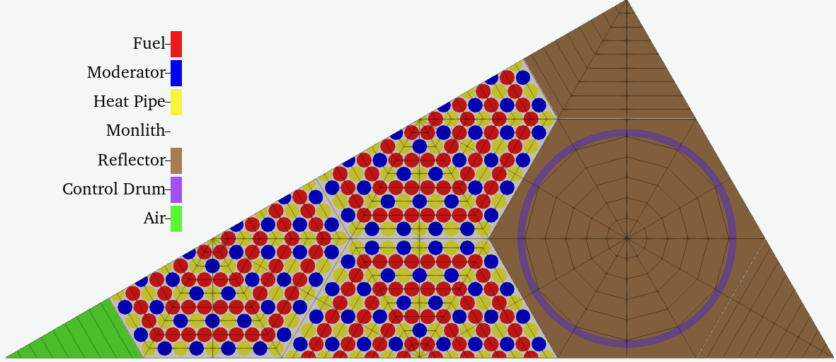
Figure 1: Coarse mesh used for assigning "coarse_element_id".
Finally, the mesh is scaled to meters and side sets are added to the mesh so that boundary conditions for thermal conduction can be properly applied:
Listing 7: Scaling the mesh and adding boundaries to the mesh.
[Mesh]
  [scale]
    type = TransformGenerator
    input = assign_coarse_elem_id
    transform = SCALE
    vector_value = '0.01 0.01 0.01'
  []

  [add_sideset_hp]
    type = SideSetsBetweenSubdomainsGenerator
    input = scale
    primary_block = '8' # add 16 so the HP boundary extends into the upper axial reflector
    paired_block = '7'
    new_boundary = 'hp'
  []

  [add_sideset_inner_mod_gap]
    type = SideSetsBetweenSubdomainsGenerator
    input = add_sideset_hp
    primary_block = '4'
    paired_block = '5'
    new_boundary = 'gap_mod_inner'
  []

  [add_sideset_outer_mod_gap]
    type = SideSetsBetweenSubdomainsGenerator
    input = add_sideset_inner_mod_gap
    primary_block = '8'
    paired_block = '5'
    new_boundary = 'gap_mod_outer'
  []
[]The resulting mesh is shown in Figure 2.
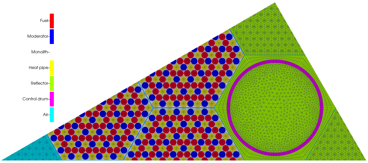
Figure 2: Fine mesh used for control drum rotation transient.
We also show the coarse element id in Figure 3.
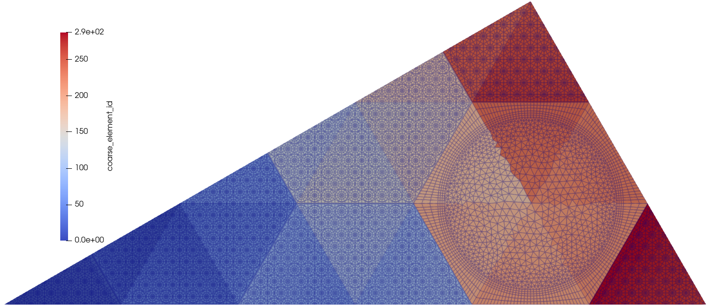
Figure 3: "coarse_element_id" on the mesh.
A list of all the blocks is shown in Table 1.
Table 1: Description of blocks in geometry
| Region | Block IDs | Multigroup cross section library ID | Solid |
|---|---|---|---|
| Fuel | 1 2 | 1001 | Yes |
| Moderator | 3 4 | 1002 | Yes |
| Moerator gap | 5 | 1002 | No |
| Heat Pipes | 6 7 | 1004 | No |
| Monolith | 8 | 1003 | Yes |
| Reflector | 10 11 14 15 | 1005 | Yes |
| Control Drum | 13 | 1005/1006 | Yes |
| Air | 20 21 | 1007 | No |
| Air | 22 | 1007 | Yes |
- Block 5 is the gap between the moderator and the monolith and filled with moderator for neutronics.
A list of all the boundaries is shown in Table 2.
Table 2: Description of boundaries in geometry
| Boundary name | Boundary description | Boundary IDs |
|---|---|---|
| bottom | bottom core boundary | 30502 |
| topleft | top-left core boundary | 30503 |
| right | right core boundary | 30504 |
| hp | Monolith-to-heat-pipe interface | 30505 |
| gap_mod_inner | Interface between moderator and air gap | 30506 |
| gap_mod_outer | Interface between monolith and air gap | 30507 |
Materials
Cross Sections
Serpent (v. 2.1.32) was used to generate the multigroup cross sections for the SiMBA problem. The ENDF/B-VIII.0 continuous energy library was utilized to leverage the scattering libraries, which was then converted into an 11-group structure to perform the calculations. The cross sections were parametrized with respect to three variables: (1) fuel temperature; (2) moderator, monolith, heat pipe, and reflector temperature; and (3) control drum angle. The grid points selected can be seen in the multigroup cross-section library file:
Listing 8: Cross section tabulation grid
version https://git-lfs.github.com/spec/v1
oid sha256:d704a72ef28147e085db911e5859e9a34e87f694d0f22a9d670c2a1ae9410121
size 1189624
The cross sections are then loaded and applied to neutronics materials, namely CoupledFeedbackNeutronicsMaterial. Auxiliary variables are also added that represent the grid variables.
Listing 9: Neutronics materials
[AuxVariables]
  [Tfuel]
    # fuel temperature
    initial_condition = 1000
  []
  [Tmod]
    # moderator + monolith + HP + reflector temperature
    initial_condition = 1000
  []
  [CD]
    # drum angle (0 = fully in, 180 = fully out)
  []
[]

[GlobalParams]
  library_file = empire_core_modified_11G_CD.xml
  library_name = empire_core_modified_11G_CD
  densities = 1.0
  isotopes = 'pseudo'
  dbgmat = false
  grid_names = 'Tfuel Tmod CD'
  grid_variables = 'Tfuel Tmod CD'
  is_meter = true
[]

[Materials]
  [fuel]
    type = CoupledFeedbackMatIDNeutronicsMaterial
    block = '1 2'
    plus = true
  []
  [non_fuel]
    type = CoupledFeedbackMatIDNeutronicsMaterial
    block = '3 4 5 6 7 8 10 11 14 15 20 21 22'
  []
  [drum]
    type = CoupledFeedbackRoddedNeutronicsMaterial
    block = '13'
    front_position_function = drum_fun
    rotation_center = '${x_center} ${y_center} 0'
    rod_segment_length = '270 90'
    segment_material_ids = '1005 1006'
    isotopes = 'pseudo; pseudo'
    densities = '1.0 1.0'
  []
[]Note the exception for the material type in the drum region. Here, we use CoupledFeedbackRoddedNeutronicsMaterial, which is material specifically for dealing with control drum and rod movement. The position of the drum is controlled by the front_position_function parameter, which accepts the name of a MOOSE Function dependent on time. Typically, three functions are defined: (1) the offset between what the actual position and what the user defines as the position, (2) a user-defined position as a function of time, and (3) combining the offset and position. For the steady-state input, these functions are constant:
Listing 10: Defining control drum position
[Functions]
  [offset]
    type = ConstantFunction
    value = 225
  []
  [drum_position]
    type = ConstantFunction
    value = 90
  []
  [drum_fun]
    type = ParsedFunction
    expression = 'drum_position + offset'
    symbol_names = 'drum_position offset'
    symbol_values = 'drum_position offset'
  []
[]

[AuxKernels]
  [CD_aux]
    type = FunctionAux
    variable = CD
    function = drum_position
    execute_on = 'initial timestep_end'
  []
[]This rodded material implements the cusping treatment described in Schunert et al. (2019). However, a significant cusping effect can still be seen in the calculated power and reactivity. Investigations indicate that the cusping effect is due to the discretization when the cross sections of the absorbing material and the non-absorbing material are significantly different. To mitigate the cusping effect, we turned on the decusping syntax by increasing the spatial expansion order (p-refinement) or refining the local elements (h-refinement) in the drum regions (automatically detected by Griffin based on the types of materials).
Listing 11: Decusping for control drum rotation.
[Decusping]
  level = 1
  switch_h_to_p_refinement = true
[]The default value for the parameter switch_h_to_p_refinement is true, meaning Griffin will perform local p-refinement for decusping. We explicitly add it here to show the existence of this parameter and users can choose h-refinement by setting this parameter to false. When this parameter is true, libMesh requires the mesh in the same order of the maximum local p-refinement order, thus we must also set second_order in the Mesh input block to true. It is often useful debug the offset by creating a simplified input that has drum position outputted to exodus. This can be done using the following debug option:
Listing 12: Debug option for outputting drum position
[Debug]
  show_rodded_materials_average_segment_in = segment_id
[]Thermal Properties
The following lists the thermal properties used for this model:
Table 3: Thermal properties
| Region | Density (kg/m) | Conductivity (W/m-K) | Specific Heat Capacity (J/kg-K) |
|---|---|---|---|
| Fuel | 14,300 | 19 | 300 |
| Moderator | 4,300 | 20 | 300 |
| Monolith | 1,800 | 70 | 1,830 |
| Reflector | 1,853.76 | 200 | 1,825 |
| Absorber | 2,520 | 20 | 1,000 |
These properties are applied using HeatConductionMaterial and GenericConstantMaterial:
Listing 13: Thermal materials
[Materials]
  #### DENSITY #####
  # units of kg/m^3
  [fuel_density]
    type = GenericConstantMaterial
    block = '${fuel_blocks}'
    prop_names = 'density'
    prop_values = 14.3e3 # same as in Serpent input
  []
  [moderator_density]
    type = GenericConstantMaterial
    block = '${moderator_blocks}'
    prop_names = 'density'
    prop_values = 4.3e3 # same as in Serpent input
  []
  [monolith_density]
    type = GenericConstantMaterial
    block = '${monolith_blocks}'
    prop_names = 'density'
    prop_values = 1.8e3 # same as in Serpent input
  []
  [reflector_density]
    type = GenericConstantMaterial
    block = '${reflector_blocks}'
    prop_names = 'density'
    prop_values = 1.85376e3 # same as in Serpent input
  []

  ### THERMAL CONDUCTIVITY ###
  # units of W/m-K
  [fuel_kappa]
    type = HeatConductionMaterial
    block = '${fuel_blocks}'
    # temperature = Tsolid
    thermal_conductivity = 19 # W/m/K
    specific_heat = 300 # reasonable value
  []
  [moderator_kappa]
    type = HeatConductionMaterial
    block = '${moderator_blocks}'
    # temperature = Tsolid
    thermal_conductivity = 20 # W/m/K
    specific_heat = 500 # random value
  []
  [monolith_thermal_props]
    type = HeatConductionMaterial
    block = '${monolith_blocks}'
    # temperature = Tsolid
    thermal_conductivity = 70 # typical value for G348 graphite
    specific_heat = 1830 # typical value for G348 graphite
  []
  [reflector_kappa]
    type = HeatConductionMaterial
    block = '${reflector_blocks}'
    # temperature = Tsolid
    thermal_conductivity = 200 # W/m/K, typical value for Be
    specific_heat = 1825 # typical value for Be
  []
  [drum_segment_props]
    type = GenericConstantMaterial
    block = '${drum_blocks}'
    prop_names = 'seg1_rho seg1_k seg1_dkdt seg1_cp
                  seg2_rho seg2_k seg2_dkdt seg2_cp'
    prop_values = '1.85376e3 200 0 1825
                   2.52e3    20  0 1000'
  []
  [drum_props]
    type = ControlDrumMaterial
    block = '${drum_blocks}'
    drum_material_properties = 'density thermal_conductivity thermal_conductivity_dT specific_heat'
    rotation_centers = '${x_center} ${y_center} 0'
    rotation_angle_functors = drum_position
    segment_angles = '270 90'
    segment_material_properties = 'seg1_rho  seg2_rho;
                                   seg1_k    seg2_k;
                                   seg1_dkdt seg2_dkdt;
                                   seg1_cp   seg2_cp'
  []
[]Since the materials in the drum region change based on the position of the control drum, ControlDrumMaterial is used to set all these properties. Based on the drum position (provided by a post-processor values received from the main application), these materials choose one of the properties of all segments on local quadrature points by which segment of the control drum they are located, either absorber or graphite.
Physics
Neutronics Physics
For this model, DFEM-SN discretization is used for the neutronics. The angular quadrature uses Gauss-Chebyshev collocation with two polar angles and six azimuthal angles. There are six delayed neutron precursors (evident from multigroup cross-section library) and first-order scattering. The physics for the neutronics is setup using the TransportSystems syntax in Griffin:
Listing 14: Defining the physics in the neutronics input
[TransportSystems]
  equation_type = eigenvalue
  particle = neutron
  G = 11

  ReflectingBoundary = 'bottom topleft'
  VacuumBoundary = 'right'

  [sn]
    scheme = DFEM-SN
    n_delay_groups = 6
    family = MONOMIAL
    order = FIRST
    AQtype = Gauss-Chebyshev
    NPolar = 2
    NAzmthl = 6
    NA = 1
  []
[]The initial power for this model is 2 MWth. Due to the 1/12th 2D geometry, this power equations to 83.333 kW/m in the simulation. The PowerDensity syntax in griffin adds an auxiliary variable for the computed power density field:
Listing 15: Power density evaluation
[PowerDensity]
  power = '${fparse 2e6 / 12 / 2}' # power: 2e6 W / 12 / 2 m (axial)
  power_density_variable = power_density
  integrated_power_postprocessor = integrated_power
  evaluate_power_density_on = 'initial timestep_end'
[]Thermal Physics
The heat conduction problem is only solved on the solid portions of the domain, i.e. excluding heat pipes, air, and moderator gaps. As such the system variable is restricted to these blocks, which requires removing some default checks in the problem:
Listing 16: Block restricted variable in thermal input
[Variables]
  [Tsolid]
    initial_condition = 950
    block = '${solid_blocks}'
  []
[]

[Problem]
  kernel_coverage_check = false
  material_coverage_check = false
[]The volumetric kernels are quite simple, including heat conduction in the solid regions and a source applied in the fuel region from the power density:
Listing 17: Thermal input volumetric kernels
[Kernels]
  [heat_conduction]
    type = HeatConduction
    variable = Tsolid
    block = '${solid_blocks}'
  []
  [heat_source_fuel]
    type = CoupledForce
    variable = Tsolid
    block = '${fuel_blocks}'
    v = power_density
  []
[]The convective heat transfer into the heat pipes is applied as a boundary condition, while the moderator gaps use GapHeatTransfer:
Listing 18: Side-set heat transfer
[BCs]
  [hp_bc]
    type = CoupledConvectiveHeatFluxBC
    variable = Tsolid
    boundary = 'hp' # inside of heat pipe
    htc = htc_hp_var
    T_infinity = Tsink_hp_var # eventually, will be given by Sockeye
  []
  [rrefl_bc]
    type = CoupledConvectiveHeatFluxBC
    variable = Tsolid
    boundary = 'right' # reflector cooling
    htc = 50 # arbitrary (but small) HTC
    T_infinity = 500 # arbitrary Tsink
  []
[]

[AuxVariables]
  [power_density]
    block = '${fuel_blocks}'
    family = MONOMIAL
    order = FIRST
    initial_condition = 2.3e6
  []
  [htc_hp_var]
    block = '${monolith_blocks}'
    initial_condition = 3e2
  []
  [Tsink_hp_var]
    block = '${monolith_blocks}'
    initial_condition = 900
  []
[]

[ThermalContact]
  [RPV_gap]
    type = GapHeatTransfer
    gap_geometry_type = 'PLATE'
    emissivity_primary = 0.8
    emissivity_secondary = 0.8 # varies from 0.6 to 1.0 in RPV paper, 0.79 in NRC paper
    variable = Tsolid # graphite -> rpv gap
    primary = 'gap_mod_inner'
    secondary = 'gap_mod_outer'
    gap_conductivity = 0.08 # W/m/K, typical thermal connectivity for air at 1000C
    quadrature = true
  []
[]Coupling
The coupling between the neutronics and thermal inputs utilize the MultiApps and Transfers systems. For this model, the neutronics serves as the main application. For steady-state, the thermal sub-application is defined as a FullSolveMultiApp:
Listing 19: Steady-state multiapp block
[MultiApps]
  [bison]
    type = FullSolveMultiApp
    input_files = thermal_ss.i
    execute_on = 'timestep_end'
    no_restore = true
    clone_parent_mesh = true
  []
[]Power density and drum position are transferred to the sub-application and temperatures are retrieved. Power density simply uses a MultiAppCopyTransfer, which directly copies the degrees of freedom of the variable from the main application to the sub-application. The drum position is computed as a post-processor, where the data is transferred via MultiAppReporterTransfer. Since the cross sections are tabulated with separate temperatures for fuel and non-fuel. However, these variables must be defined everywhere in order to evaluate the cross sections. To do this, we use MultiAppGeneralFieldNearestLocationTransfer that is block restricted on the sub-application side. This transfer will then do a direct degree a freedom transfer for Tfuel in the fuel region and extrapolate from the nearest node in the non-fuel region. The same goes for Tmod in the non-fuel vs. fuel regions.
Listing 20: Variable transfers
[Transfers]
  [pdens_to_modules]
    type = MultiAppCopyTransfer
    to_multi_app = bison
    source_variable = power_density
    variable = power_density
  []
  [dp_to_modules]
    type = MultiAppReporterTransfer
    to_multi_app = bison
    from_reporters = dp/value
    to_reporters = drum_position/value
  []
  [tfuel_from_modules]
    type = MultiAppGeneralFieldNearestLocationTransfer
    from_multi_app = bison
    variable = Tfuel
    source_variable = Tsolid
    from_blocks = '1 2'
    # Values are transferred outside the block restriction of Tfuel, leading to some indetermination
    search_value_conflicts = false
    # Reduces transfers efficiency for now, can be removed once transferred fields are checked
    bbox_factor = 10
  []
  [tmod_from_modules]
    type = MultiAppGeneralFieldNearestLocationTransfer
    from_multi_app = bison
    variable = Tmod
    source_variable = Tsolid
    from_blocks = '3 4 8 10 11 13 14 15 22'
    search_value_conflicts = false
    # Reduces transfers efficiency for now, can be removed once transferred fields are checked
    bbox_factor = 10
  []
[]Solvers
Griffin utilizes a customized executioner for DFEM-SN systems known as SweepUpdate. See this Griffin tutorial for more details on the methodology.
Listing 21: Griffin executioner for steady-state DFEM-SN with CMFD
[Executioner]
  type = SweepUpdate

  fixed_point_solve_outer = true
  custom_pp = eigenvalue
  fixed_point_max_its = 50
  custom_rel_tol = 1e-6

  richardson_rel_tol = 1e-1
  richardson_abs_tol = 1e-4
  richardson_max_its = 100
  richardson_value = eigenvalue
  inner_solve_type = GMRes
  max_inner_its = 2

  cmfd_acceleration = true
  coarse_element_id = coarse_element_id
  prolongation_type = multiplicative
  max_diffusion_coefficient = 1
  diffusion_n_free_power_its = 0
  diffusion_newton_rel_tol = 1e-3
[]The thermal application simply uses the traditional Steady executioner, which specifies using AMG to speed up convergence.
Listing 22: Executioner for steady-state thermal problem
[Executioner]
  type = Steady
  petsc_options_iname = '-pc_type -pc_hypre_type -ksp_gmres_restart'
  petsc_options_value = 'hypre boomeramg 300'
  line_search = 'none'

  l_tol = 1e-02
  nl_abs_tol = 1e-7
  nl_rel_tol = 1e-8

  l_max_its = 50
  nl_max_its = 25
[]Transient
Initial Conditions
For this model, the initial condition comes from the steady-state solution. This solution is written to a binary file and loaded in the transient simulation using SolutionVectorFile and TransportSolutionVectorFile. The steady-state solution is written by adding the user-objects to the steady-state inputs, with the important parameter specification: execute_on = FINAL.
Listing 23: Writing steady-state neutronics solution to a file
[UserObjects]
  [neutronics_initial]
    type = TransportSolutionVectorFile
    transport_system = sn
    folder = 'binary_90'
    execute_on = final
  []
  [neutronics_thermal_initial]
    type = SolutionVectorFile
    var = 'Tfuel Tmod'
    folder = 'binary_90'
    execute_on = final
  []
[]Listing 24: Writing steady-state thermal solution to a file
[UserObjects]
  [thermal_initial]
    type = SolutionVectorFile
    var = 'Tsolid power_density'
    folder = 'binary_90'
    execute_on = final
  []
[]The files are loaded with the same objects (must also be the same name) with parameters: writing = false and execute_on = INITIAL.
Listing 25: Loading steady-state neutronics solution from file
[UserObjects]
  [neutronics_initial]
    type = TransportSolutionVectorFile
    transport_system = sn
    folder = 'binary_90'
    writing = false
    execute_on = initial
  []
  [neutronics_adjoint]
    type = TransportSolutionVectorFile
    folder = 'binary_90'
    transport_system = sn
    writing = false
    load_to_adjoint = true
    disable_eigenvalue_transfer = true
    execute_on = initial
  []
  [neutronics_thermal_initial]
    type = SolutionVectorFile
    var = 'Tfuel Tmod'
    folder = 'binary_90'
    writing = false
    execute_on = initial
  []
[]Listing 26: Loading steady-state thermal solution from file
[UserObjects]
  [thermal_initial]
    type = SolutionVectorFile
    var = 'Tsolid power_density'
    folder = 'binary_90'
    writing = false
    execute_on = initial
  []
[]Adjoint Problem
In order to compute point-kinetics parameters, like dynamic reactivity and mean generation time, Griffin requires the computation of an adjoint solution. This is done by running the adjoint version of the steady-state neutronics input. The adjoint input is basically the same as the forward input, with a couple key differences. First, the problem is de-coupled, so there are not MultiApps or Transfers and the thermal solution is loaded from forward solution file. Second, TransportSystems must have the parameter for_adjoint = true set.
Listing 27: Neutronics adjoint problem
[UserObjects]
  [neutronics_adjoint]
    type = TransportSolutionVectorFile
    transport_system = sn
    folder = 'binary_90'
    execute_on = final
  []
  [neutronics_thermal_initial]
    type = SolutionVectorFile
    folder = 'binary_90'
    var = 'Tfuel Tmod'
    writing = false
    execute_on = initial
  []
[]

[TransportSystems]
  equation_type = eigenvalue
  particle = neutron
  G = 11

  ReflectingBoundary = 'bottom topleft'
  VacuumBoundary = 'right'

  for_adjoint = true
  [sn]
    scheme = DFEM-SN
    n_delay_groups = 6
    family = MONOMIAL
    order = FIRST
    AQtype = Gauss-Chebyshev
    NPolar = 2
    NAzmthl = 6
    NA = 1
  []
[]Neutronics Transient
The transient input for neutronics is largely identical to the steady-state version. The following presents the key differences. First, equation_type = transient in the TransportSystems block must be set. Second, function describing the control drum position now depends on time. Third, the multi-app for the thermal sub-application is now a TransientMultiApp.
Listing 28: Changes for neutronics transient input
[TransportSystems]
  equation_type = transient
  particle = neutron
  G = 11

  ReflectingBoundary = 'bottom topleft'
  VacuumBoundary = 'right'

  [sn]
    scheme = DFEM-SN
    n_delay_groups = 6
    family = MONOMIAL
    order = FIRST
    AQtype = Gauss-Chebyshev
    NPolar = 2
    NAzmthl = 6
    NA = 1
    dnp_amp_scheme = quadrature
  []
[]

[Functions]
  [offset]
    type = ConstantFunction
    value = 225
  []
  [drum_linear]
    type = ParsedFunction
    expression = 'if(t <= t_out, pos_start + speed * t, (pos_start + speed * t_out) - speed * (t - t_out))'
    symbol_names = 't_out pos_start speed'
    symbol_values = '${t_out} ${pos_start} ${speed}'
  []
  [drum_position]
    type = ParsedFunction
    expression = 'if(drum_linear < 0, 0, if(drum_linear > 180, 180, drum_linear))'
    symbol_names = 'drum_linear'
    symbol_values = 'drum_linear'
  []
  [drum_fun]
    type = ParsedFunction
    expression = 'drum_position + offset'
    symbol_names = 'drum_position offset'
    symbol_values = 'drum_position offset'
  []
[]

[MultiApps]
  [bison]
    type = TransientMultiApp
    input_files = thermal_transient.i
    execute_on = 'timestep_end'
    clone_parent_mesh = true
  []
[]Finally, the executioner is changed to IQSSweepUpdate, which utilized the improved quasi-static method (IQS). The algorithm this executioner implements is described in detail in Prince et al. (2023). The pke_param_csv = true parameter triggers an output of point kinetics parameters and output_micro_csv = true outputs the detailed power profile of the transient.
Listing 29: Neutronics solver using IQS
[Executioner]
  type = IQSSweepUpdate
  pke_param_csv = true
  output_micro_csv = true

  end_time = 5
  # This constant timestep size has to be small enough to avoid negative solutions
  # during the transient. It is likely too fine for the beginning and the end of the
  # transient. We possibly can apply time adaptation in the future to improve the
  # performance of the transient simulations.
  dt = 0.03

  fixed_point_solve_outer = true
  fixed_point_max_its = 50
  custom_pp = integrated_power
  custom_abs_tol = 1 # W
  custom_rel_tol = 1e-6

  richardson_rel_tol = 1e-4
  richardson_abs_tol = 5e-5
  richardson_max_its = 200
  richardson_value = integrated_power
  inner_solve_type = GMRes
  max_inner_its = 2

  cmfd_acceleration = true
  coarse_element_id = coarse_element_id
  prolongation_type = multiplicative
  max_diffusion_coefficient = 1
[]We use a simple constant time step size for this transient. Numerical results indicate that the time step size needs to be smaller than a threshold to avoid negative solutions close to the peak power. A better time-stepping scheme with time adaptation can possibly applied in the future.
Thermal Transient
Again, the transient input of the thermal model is largely the same as the steady-state input. First, the time derivative is added to the volumetric kernels. Second, the executioner type is changed to Transient. Note that the time stepping scheme is not included in this input, since it will be defined by the main neutronics application.
Listing 30: Changes for thermal transient input
[Kernels]
  [time_derivative]
    type = HeatConductionTimeDerivative
    variable = Tsolid
    block = '${solid_blocks}'
  []
  [heat_conduction]
    type = HeatConduction
    variable = Tsolid
    block = '${solid_blocks}'
  []
  [heat_source_fuel]
    type = CoupledForce
    variable = Tsolid
    block = '${fuel_blocks}'
    v = power_density
  []
[]

[Executioner]
  type = Transient

  petsc_options_iname = '-pc_type -pc_hypre_type -ksp_gmres_restart'
  petsc_options_value = 'hypre boomeramg 300'
  line_search = 'none'

  l_tol = 1e-02
  nl_abs_tol = 1e-7
  nl_rel_tol = 1e-8

  l_max_its = 50
  nl_max_its = 25
[]Running Model
This model can be run using a Griffin executable, or any application built with Griffin (BlueCRAB, Direwolf, etc.). The simulations scale decently well, so either a workstation or HPC can be used. The following presents the commands used to run the model and produce results. They must be executed in this order and with the same number of processors. Run times are presented at various processor counts, which were obtained by running the simulations on the INL Bitterroot cluster with one computing node.
First is building the meshes, which produces empire_2d_CD_fine_in.e:
griffin-opt -i empire_2d_CD_fine.i --mesh-onlySecond is the coupled steady-state calculation, which produces neutronics_eigenvalue_out.e and neutronics_eigenvalue_out_bison0.e:
mpiexec -n <n> griffin-opt -i neutronics_eigenvalue.iWe can also run neutronics only without coupling the thermal conduction with command-line options:
mpiexec -n <n> griffin-opt -i neutronics_eigenvalue.i MultiApps/active='' Transfers/active=''MultiApps/active='' Transfers/active='' are for turning off the multiphysics coupling. Note that we still have the Picard iteration as the outer iteration. At the end of each Picard iteration, Griffin will perform some extra evaluations for auxiliary variables, postprocessors executed on timestep_end and outputs. But because inner Richardson iteration continues with the solution from the last Richardson iteration in the previous outer Picard iteration, the overall performance does not change much with only the Richardson iteration with the same number of iterations.
We also gather the run times by turning outputs off, as the outputs used in this simulation are convenient to use, but not optimized for scalability:
mpiexec -n <n> griffin-opt -i neutronics_eigenvalue.i Outputs/exodus=false UserObjects/active='' bison:UserObjects/active=''for the coupled multiphysics simulation, and
mpiexec -n <n> griffin-opt -i neutronics_eigenvalue.i MultiApps/active='' Transfers/active='' Outputs/exodus=false UserObjects/active=''for the neutronics-only runs. Run times for all four calculations with different number of processors are presented in Table 4.
Table 4: Run times for steady-state simulation on various processors
Processors (<n>) | Neutronics-only (s) | Neutronics-only no-output (s) | Multiphysics (s) | Multiphysics no-output (s) |
|---|---|---|---|---|
| 4 | 139 | 123 | 146 | 131 |
| 8 | 81 | 69 | 87 | 74 |
| 16 | 48 | 38 | 51 | 41 |
| 32 | 27 | 20 | 29 | 23 |
| 64 | 18 | 13 | 20 | 15 |
| 96 | 14 | 10 | 17 | 12 |
Third is the adjoint neutronics calculation:
mpiexec -n <n> griffin-opt -i neutronics_adjoint.iTable 5: Run times for adjoint simulation on various processors
Processors (<n>) | Run-time (s) |
|---|---|
| 4 | 113 |
| 8 | 63 |
| 16 | 35 |
| 32 | 19 |
| 64 | 12 |
| 96 | 9 |
Finally, the coupled transient can be run, which produces several output files which can be postprocessed:
neutronics_transient_out.e: Contains neutronics-evaluated quantities like power density and scalar flux shape. Note that the scalar flux shape must be scaled by the power scaling factor and IQS amplitude to retrieve the actual flux.neutronics_transient_out_bison0.e: Contains thermal-evaluated quantities such as the temperature field.neutronics_transient_out.csv: Contains global neutronics-evaluated quantities, like power.neutronics_transient_out_bison0.csv: Contains global thermal-evaluated quantities, like average and max temperatures.neutronics_transient_out_pke_params.csv: Contains point-kinetics parameters, like reactivity.neutronics_transient_out_micro_power.csv: Contains the flux amplitude, which can be used obtain a detailed temporal profile of the power.
mpiexec -n <n> griffin-opt -i neutronics_transient.iTable 6: Run times for adjoint simulation on various processors
Processors (<n>) | Run-time (min) |
|---|---|
| 4 | 743 |
| 8 | 432 |
| 16 | 250 |
| 32 | 136 |
| 64 | 84 |
| 96 | 62 |
A single transient simulation includes 167 time steps with a total of 4,381 Richardson iterations.
Results
The full transient profile of power, average and maximum temperatures, and reactivity are shown in Figure 4, Figure 5 and Figure 6 respectively.

Figure 4: Transient power profile.

Figure 5: Transient temperature profile.

Figure 6: Transient reactivity profile.
These plots show that during the first second, the transient is purely kinetics driven as reactivity from rotating the control drum outward into the core. Maximum power is reached around 1.41 seconds. The core temperatures rise significantly at this point, causing the power to drop due to the negative temperature feedback in the fuel, even while the drum is still rotating outward. The power drops exponentially as the drums are rotated back inward, causing the temperatures to flatten and eventually drop due to heat removal.
The following results were produced before we updated the model with the latest drum rotation decusping treatment. The update mainly affects the performance and does not change the results significantly, thus the presented results are still representative.
The initial temperature and power profile are shown in Figure 7. The full transient profile of power, average and maximum temperatures, and reactivity are shown in Figure 8. These plots show that during the first second, the transient is purely kinetics driven as reactivity from rotating the control drum outward into the core. Maximum power is reached around 1.25 seconds. The core temperatures rise significantly at this point, causing the power to drop due to the negative temperature feedback in the fuel, even while the drum is still rotating outward. The power drops exponentially as the drums are rotated back inward, causing the temperatures to flatten and eventually drop due to heat removal. The spatial profile of the power density and temperature during the transient are shown in Figure 9.
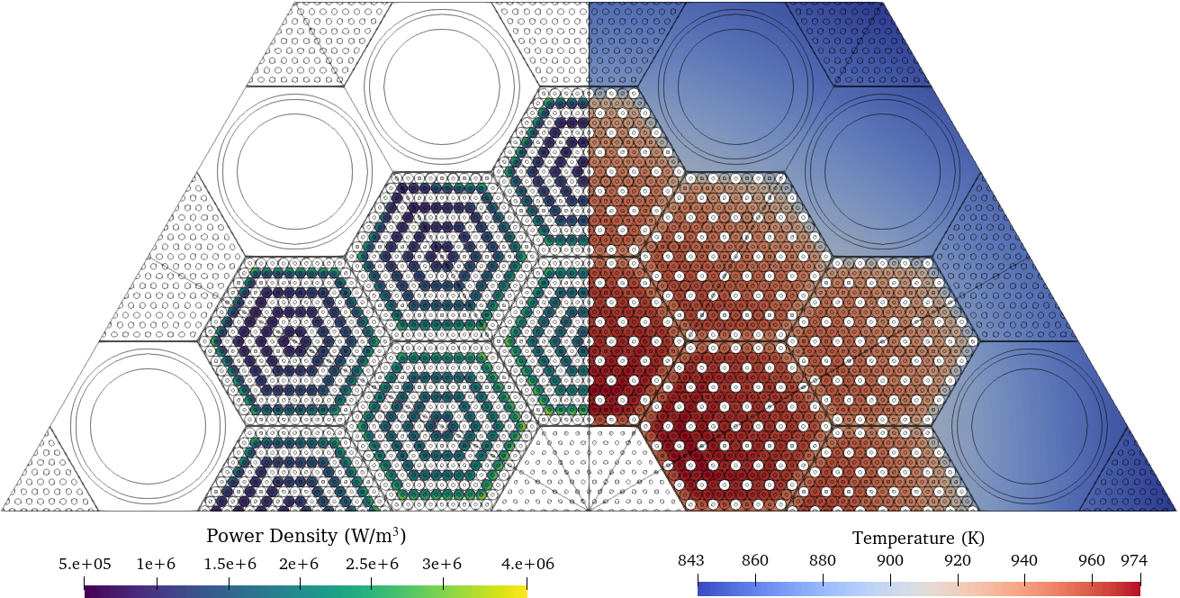
Figure 7: Initial power and temperature profile
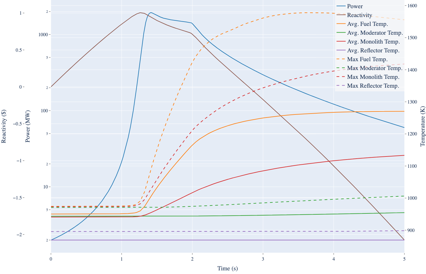
Figure 8: Values of selected quantities over simulated transient for control drum rotation.
Figure 9: Power density and temperature fields over transient
References
- Christopher Matthews, Vincent Laboure, Mark DeHart, Joshua Hansel, David Andrs, Yaqi Wang, Javier Ortensi, and Richard C Martineau.
Coupled multiphysics simulations of heat pipe microreactors using direwolf.
Nuclear Technology, 207(7):1142–1162, 2021.[Export]
- Zachary Prince, Joshua Hanophy, Vincent Labouré, Yaqi Wang, Logan Harbour, and Namjae Choi.
Neutron transport methods for multiphysics heterogeneous reactor core simulation in griffin.
Submitted to Annals of Nuclear Energy, 2023.[Export]
- Sebastian Schunert, Yaqi Wang, Javier Ortensi, Vincent Laboure, Frederick Gleicher, Mark DeHart, and Richard Martineau.
Control rod treatment for FEM based radiation transport methods.
Annals of Nuclear Energy, 127:293–302, May 2019.
doi:10.1016/j.anucene.2018.11.054.[Export]
- Stefano Terlizzi and Vincent Labouré.
Asymptotic hydrogen redistribution analysis in yttrium-hydride-moderated heat-pipe-cooled microreactors using direwolf.
Annals of Nuclear Energy, 186:109735, 2023.
URL: https://www.sciencedirect.com/science/article/pii/S0306454923000543, doi:https://doi.org/10.1016/j.anucene.2023.109735.[Export]