3D Stress Analysis
This page discusses the model set-up for the stress analysis of a 3D MSRE graphite stringer subject to an user-defined infiltration amount, by using the reference solution file generated for this geometry.
Computational Model Description
Figure 1 shows the mesh of the unit cell of the MSRE graphite stringer.
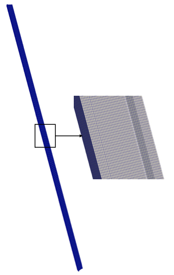
Figure 1: Finite element mesh of the 3D unit cell of the graphite stringer.
Files used by this model include:
MOOSE input file
Exodus mesh file
CSV file defining the variation of the coolant temperature and volumetric heat
Exodus reference solution file for initializing the infiltration amount
This document reviews the inportant elements of the input file that were not covered in previous infiltration models (creation of infiltration profiles and creation of a reference solution file), listed in full here:
# ==============================================================================
# Input file to predict stresses due to a specified infiltration amount
# Application : MOOSE
# ------------------------------------------------------------------------------
# Idaho Falls, INL, 2025
# Author(s): V Prithivirajan, Ben Spencer
# If using or referring to this model, please cite as explained on
# https://mooseframework.inl.gov/virtual_test_bed/citing.html
# ==============================================================================

### INPUTS ###

E = 9.8e9    #Pa
K = 63.      #W/mK
nu = 0.14
htc = 4500   #W/m^2K
CTE = 4.5e-6 #1/K

volume_fraction = 0.33
threshold = 0.8

[GlobalParams]
  displacements = 'disp_x disp_y disp_z'
[]

[Mesh]
  file = '../1_create_infiltration_profile/3D/msre3D_0PF_Fine.e'
[]

[Variables]
  [T]
    initial_condition = 300.0 #K
  []
[]

[AuxVariables]
  [T_inf]
  []
  [smooth_read]
    order = FIRST
    family = LAGRANGE
  []
[]

[Functions]
  [volumetric_heat] #Axial distribution of the power density
    type = PiecewiseLinear
    data_file = interpolated_T_PD_values.csv
    x_index_in_file = 0
    y_index_in_file = 2
    format = columns
    xy_in_file_only = false
    axis = z
  []
  [T_infinity_fn] #Temperature distribution at the graphite-coolant interface
    type = PiecewiseLinear
    data_file = interpolated_T_PD_values.csv
    x_index_in_file = 0
    y_index_in_file = 5
    format = columns
    xy_in_file_only = false
    axis = z
  []
  [heatsource_soln_func] #Infiltration profile corresponding to user-defined amount
    type = SolutionFunction
    solution = heatsource_soln
    from_variable = diffuse
  []
  [bin_heatsource_soln_func] #Binarize heatsource_soln_func
    type = ParsedFunction
    symbol_names = smooth_mod
    symbol_values = heatsource_soln_func
    expression = 'if(smooth_mod>=${threshold},1,0)'
  []
  [mod_heatsource_soln_func] #Obtain 3D distribution of the power density
    type = ParsedFunction
    symbol_names = 'bin_heatsource_soln_func volumetric_heat'
    symbol_values = 'bin_heatsource_soln_func volumetric_heat'
    expression = bin_heatsource_soln_func*volumetric_heat
  []
[]

[Kernels]
  [heat_conduction]
    type = HeatConduction
    variable = T
  []
  [heat_source]
    type = HeatSource
    variable = T
    function = mod_heatsource_soln_func
  []
[]

[AuxKernels]
  [T_inf]
    type = FunctionAux
    variable = T_inf
    function = T_infinity_fn
    execute_on = initial
  []
  [smooth_read_fn]
    type = FunctionAux
    variable = smooth_read
    function = mod_heatsource_soln_func
    execute_on = TIMESTEP_BEGIN
  []
[]

[Physics]

  [SolidMechanics]

    [QuasiStatic]
      [all]
        add_variables = true
        strain = small
        automatic_eigenstrain_names = true
        generate_output = 'stress_xx stress_yy max_principal_stress vonmises_stress'
        material_output_order = FIRST
        material_output_family = LAGRANGE
      []
    []
  []
[]

[UserObjects]
  [heatsource_soln]
    type = SolutionUserObject
    mesh = '../2_create_reference_solution_file/gold/CombinedExodus_AllResults_out.e'
    time_transformation = ${volume_fraction}
    system_variables = 'diffuse'

    # For testing only : turning 3D into 2D when mapping into the UO
    scale_multiplier = '1 1 0'
    transformation_order = 'scale_multiplier'
  []
[]

[Materials]
  [thermal]
    type = HeatConductionMaterial
    thermal_conductivity = ${K}
    specific_heat = 1400 #J/KgK
  []
  [density]
    type = GenericConstantMaterial
    prop_names = 'density'
    prop_values = 1760.0 #Kg/m^3
  []
  [elasticity]
    type = ComputeIsotropicElasticityTensor
    youngs_modulus = ${E}
    poissons_ratio = ${nu}
  []
  [expansion1]
    type = ComputeThermalExpansionEigenstrain
    temperature = T
    thermal_expansion_coeff = ${CTE}
    stress_free_temperature = 300 #K
    eigenstrain_name = thermal_expansion
  []
  [stress]
    type = ComputeLinearElasticStress
  []
[]

[BCs]
  [xsymm_left]
    type = DirichletBC
    variable = disp_x
    value = 0
    boundary = 'XMINUS'
  []
  [ysymm_bottom]
    type = DirichletBC
    variable = disp_y
    value = 0
    boundary = 'YMINUS'
  []

  [zsymm_bottom]
    type = DirichletBC
    preset = true
    variable = disp_z
    value = 0
    boundary = 'ZMINUS'
  []

  [convective_heat_transfer]
    type = CoupledConvectiveHeatFluxBC
    variable = T
    boundary = 'coolantchannelboundary'
    T_infinity = T_inf
    htc = ${htc}
  []
[]

[Postprocessors]
  [maxstress]
    type = ElementExtremeValue
    variable = max_principal_stress
    value_type = max
  []
[]
[VectorPostprocessors]
  [line]
    type = LineValueSampler
    start_point = '0 0 1.6637'
    end_point = '0.0148 0.0139 0'
    num_points = 100
    sort_by = 'z'
    variable = 'disp_x disp_y disp_z T'
    execute_on = timestep_end
  []
[]

[Preconditioning]
  [smp]
    type = SMP
    full = true
  []
[]

[Executioner]
  type = Steady
  solve_type = 'NEWTON'
  petsc_options_iname = '-pc_type -pc_hypre_type -pc_hypre_boomeramg_strong_threshold'
  petsc_options_value = 'hypre    boomeramg      0.6'
  line_search = 'none'
  nl_abs_tol = 1.0e-10
  nl_rel_tol = 1.0e-08
[]

[Outputs]
  checkpoint = false
  csv = true
[]Initializing inputs from CSV file
Two quantities, namely, the volumetric heat (volumetric_heat) and the coolant temperature (T_infinity_fn) are read from the CSV file. These values are then used to construct piecewise linear functions for both quantities along the z-axis.
[Functions]
  [volumetric_heat]
    #Axial distribution of the power density
    type = PiecewiseLinear
    data_file = interpolated_T_PD_values.csv
    x_index_in_file = 0
    y_index_in_file = 2
    format = columns
    xy_in_file_only = false
    axis = z
  []

  [T_infinity_fn]
    #Temperature distribution at the graphite-coolant interface
    type = PiecewiseLinear
    data_file = interpolated_T_PD_values.csv
    x_index_in_file = 0
    y_index_in_file = 5
    format = columns
    xy_in_file_only = false
    axis = z
  []
[]Initializing user-defined infiltration amount using the reference solution file
First, a SolutionUserObject is used to read the interpolated infiltration profile, specifically the diffuse variable, from the reference solution file named CombinedExodus_AllResults_out.e. This is done at the user-defined infiltration amount of 33%, as specfied by volume_fraction = 0.33.
[UserObjects]
  [heatsource_soln]
    type = SolutionUserObject
    mesh = '../2_create_reference_solution_file/gold/CombinedExodus_AllResults_out.e'
    time_transformation = ${volume_fraction}
    system_variables = 'diffuse'

    # For testing only : turning 3D into 2D when mapping into the UO
    scale_multiplier = '1 1 0'
    transformation_order = 'scale_multiplier'
  []
[]Following this, SolutionFunctions below obtains the data from the SolutionUserObject and makes it available as a function for the current simulation.
[Functions]
  [heatsource_soln_func]
    #Infiltration profile corresponding to user-defined amount
    type = SolutionFunction
    solution = heatsource_soln
    from_variable = diffuse
  []
[]The infiltration amount specifies the region where the volumetric heat needs to be defined. In previous steps, the infiltration profile is obtained through the diffuse variable. Here, the profile is binarized and then multiplied by the actual volumetric heat to define the required heat distribution. This is accomplished via the following block:
[Functions]
  [bin_heatsource_soln_func]
    #Binarize heatsource_soln_func
    type = ParsedFunction
    symbol_names = smooth_mod
    symbol_values = heatsource_soln_func
    expression = 'if(smooth_mod>=${threshold},1,0)'
  []

  [mod_heatsource_soln_func]
    #Obtain 3D distribution of the power density
    type = ParsedFunction
    symbol_names = 'bin_heatsource_soln_func volumetric_heat'
    symbol_values = 'bin_heatsource_soln_func volumetric_heat'
    expression = bin_heatsource_soln_func*volumetric_heat
  []
[]Solid Mechanics Action
This block defines a MOOSE Action that automates the process of setting up the solid mechanics kernel using small strain kinematics. It simplifies the set up by automatically adding displacement variables, handling eigenstrain inputs, and generating auxillary variables for key stress components. This method reduces manual setup by leveraging the solid mechanics action.
[Physics]

  [SolidMechanics]

    [QuasiStatic]
      [all]
        add_variables = true
        strain = small
        automatic_eigenstrain_names = true
        generate_output = 'stress_xx stress_yy max_principal_stress vonmises_stress'
        material_output_order = FIRST
        material_output_family = LAGRANGE
      []
    []
  []
[]Running the model
To run this model using the MOOSE combined module executable, run the following command:
mpiexec -n 100 /path/to/app/combined-opt -i msre3D_100percent_INF.i
Note: HPC resources were used to perform this simulation
The following Exodus results file will be produced: msre3D_100percent_INF_exodus.e
The Exodus output file can be visualized with Paraview.